Cracking Complex Puzzles - AI Strategies for Constraints and Competitions

Welcome back, AI aficionados! In our previous discussions, we've seen how AI agents perceive their environment and use search strategies to find solutions. But what happens when problems come with a specific set of rules or constraints? Or when an agent has to make decisions in a competitive setting, like a game?

Today, we're venturing into two fascinating areas of AI problem-solving:

1. Constraint Satisfaction Problems (CSPs): Where solutions must satisfy a given set of limitations.
2. Adversarial Search: How AI agents make optimal decisions when facing an opponent.

Get ready to unravel how AI cracks these complex puzzles!

Constraint Satisfaction Problems (CSPs): Finding Solutions Within Boundaries

Many real-world problems involve finding a state that satisfies a collection of constraints. These are known as Constraint Satisfaction Problems (CSPs).

A CSP is formally defined by three components:

• A set of variables $X_1, X_2, \dots, X_n$.
• For each variable $X_i$, a non-empty domain $D_i$ of possible values.
• A set of constraints $C_1, C_2, \dots, C_m$. Each constraint $C_i$ involves some subset of the variables and specifies the allowable combinations of values for that subset.

A state in a CSP is an assignment of values to some or all of the variables. An assignment that does not violate any constraints is called consistent or legal. A complete assignment is one where every variable is assigned a value. A solution to a CSP is a complete assignment that satisfies all constraints.

Unlike standard search problems where a state is a "black box," in CSPs, the state is defined by variables and their values, and the goal test is the set of constraints.

Example: Map-Coloring ️

A classic CSP is map coloring. The task is to color regions on a map such that no two adjacent regions have the same color.

• Variables: The regions (e.g., WA, NT, Q, NSW, V, SA, T for Australia).
• Domains: The set of available colors for each region (e.g., {red, green, blue}).
• Constraints: Adjacent regions must have different colors (e.g., WA $\neq$ NT).

A solution would be an assignment of colors to all regions that satisfies these constraints, like WA = red, NT = green, etc..

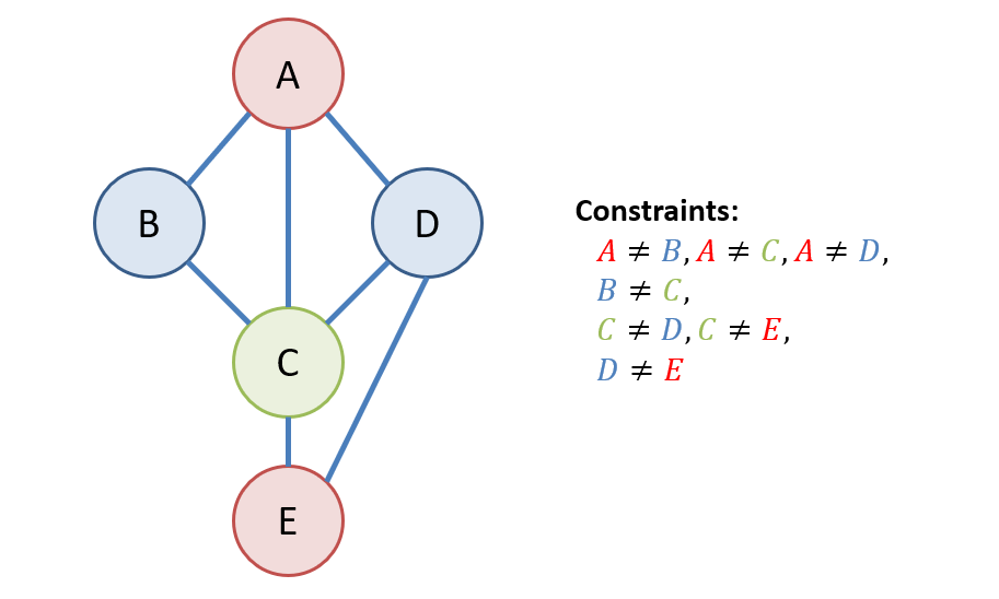(Constraint graph for the Australia map-coloring problem. Each node is a variable (region), and an arc between nodes means their colors must be different.)

For binary CSPs, where each constraint relates two variables, a constraint graph can be drawn where nodes are variables and arcs represent constraints between them.

Varieties of CSPs and Constraints

CSPs come in different flavors:

• Discrete Variables:
  • Finite Domains: The number of possible assignments is $O(d^n)$ for $n$ variables and domain size $d$. Boolean CSPs (like Boolean satisfiability) fall into this category and are often NP-complete.
  • Infinite Domains: Variables can be integers, strings, etc. (e.g., job scheduling with start/end dates). These require a constraint language (e.g., StartJob1 + 5 $\le$ StartJob3).
• Continuous Variables: Used for problems like scheduling Hubble Space Telescope observations. Linear constraints here can often be solved in polynomial time using linear programming.

Constraints also vary:

• Unary Constraints: Involve a single variable (e.g., SA $\neq$ green).
• Binary Constraints: Involve pairs of variables (e.g., SA $\neq$ WA).
• Higher-Order Constraints: Involve three or more variables (e.g., column constraints in cryptarithmetic puzzles).

Example: Cryptarithmetic

Cryptarithmetic puzzles are another common example of CSPs.

    T W O
  + T W O
  ------
    F O U R

    S E N D
  + M O R E
  ------
    M O N E Y

• Variables: F, T, U, W, R, O (in TWO + TWO = FOUR example from slides) or S, E, N, D, M, O, R, Y and carry bits $X_1, X_2, X_3$ (for SEND+MORE=MONEY).
• Domains: {0, 1, ..., 9} for each letter.
• Constraints:
  • Alldiff(letters): Each letter must have a unique digit.
  • Arithmetic constraints for each column (e.g., O + O = R + 10 * $X_1$ for TWO+TWO=FOUR, or D + E = Y + 10 * $C_1$ for SEND+MORE=MONEY ).
  • Leading letters cannot be zero (e.g., T $\neq$ 0, F $\neq$ 0 for TWO+TWO=FOUR; S $\neq$ 0, M $\neq$ 0 for SEND+MORE=MONEY ).

Real-world CSPs include assignment problems (who teaches what class), timetabling, transportation scheduling, and factory scheduling.

Backtracking Search for CSPs: A Systematic Exploration

A common algorithm for solving CSPs is backtracking search. It's a form of depth-first search where variables are assigned values one at a time, and if an assignment violates a constraint, the search backtracks to try a different value for the preceding variable.

The standard incremental search formulation defines states by the values assigned so far. The initial state is an empty assignment. The successor function assigns a value to an unassigned variable, provided it doesn't conflict with current assignments; it fails if no legal assignments exist. The goal test is when the current assignment is complete and consistent. Since variable assignments are commutative (e.g., [WA=red then NT=green] is the same as [NT=green then WA=red]), we only need to consider assignments to a single variable at each node.

Improving Backtracking Efficiency

Plain backtracking can be inefficient. Several heuristics can significantly improve its performance:

1. Which variable should be assigned next?

   • Most Constrained Variable (MRV): Choose the variable with the fewest remaining legal values. This is also called the "minimum remaining values" heuristic.
   • Most Constraining Variable (Degree Heuristic): As a tie-breaker for MRV, choose the variable that is involved in the largest number of constraints on other unassigned variables.

2. In what order should its values be tried?

   • Least Constraining Value: Prefer the value that rules out the fewest choices for the neighboring variables in the constraint graph. This tries to leave maximum flexibility for subsequent variable assignments.

3. Can we detect inevitable failure early?

   • Forward Checking: When a variable X is assigned a value, check each unassigned variable Y connected to X by a constraint. Delete any value from Y's domain that is inconsistent with the value chosen for X. If any variable has no legal values left, the search backtracks immediately.
   • Constraint Propagation (e.g., Arc Consistency): Forward checking propagates information from assigned to unassigned variables but doesn't detect all inconsistencies early. Constraint propagation repeatedly enforces constraints locally.
     • Arc Consistency: An arc X $\rightarrow$ Y is consistent if, for every value x in the domain of X, there is some allowed value y in the domain of Y. If X loses a value, its neighbors need to be rechecked. The AC-3 algorithm can enforce arc consistency. Arc consistency detects failures earlier than simple forward checking and can be run as a preprocessor or after each assignment.

These techniques make solving much larger CSPs feasible, even n-queens for large n.

Adversarial Search: Playing to Win

Now, let's shift gears to adversarial search, which deals with problems where agents compete with each other, typically in games.

Games vs. Standard Search Problems

Games differ from standard search problems in key ways:

• Unpredictable Opponent: You need a strategy that specifies a move for every possible reply from your opponent.
• Time Limits: Often, you can't search to the end of the game (the goal state). You must make the best decision within a limited time, often by approximating the value of states.

Game Search Problem Formulation

A game can be formulated as a search problem:

• Initial State: The initial board position and whose turn it is.
• Operators (Actions): The legal moves a player can make.
• Terminal Test (Goal Test): Determines if the game is over.
• Utility Function (Payoff Function): A numeric value for the outcome of the game from a player's perspective (e.g., +1 for win, 0 for draw, -1 for loss).

The objective is to find a sequence of player's decisions (moves) that maximizes its utility, considering the opponent's moves which aim to maximize their utility (and thus minimize yours in a zero-sum game).

A game tree represents all possible sequences of moves.

Optimal Decisions in Games: The Minimax Algorithm

The Minimax algorithm is designed for perfect play in deterministic, two-player games where players alternate turns and have complete information. The core idea is to choose the move leading to the position with the highest minimax value. This value represents the best achievable payoff against a rational opponent who is also playing optimally.

• MAX player: Tries to maximize the utility.
• MIN player: Tries to minimize MAX's utility (or maximize its own).

The algorithm explores the game tree:

1. Generate the game tree down to the terminal states.
2. Compute the utility of each terminal state.
3. For nodes at depth d-1, compute their values from their children's values (MAX takes the maximum, MIN takes the minimum).
4. Continue backing up values towards the root.
5. The MAX player chooses the move that leads to the highest value.

Properties of Minimax:

• Complete? Yes, if the tree is finite.
• Optimal? Yes, against an optimal opponent.
• Time Complexity? $O(b^m)$, where b is the branching factor and m is the maximum depth.
• Space Complexity? $O(bm)$ for depth-first exploration.

For games like chess (b $\approx$ 35, m $\approx$ 100), exact minimax search is completely infeasible due to the massive search space.

Alpha-Beta Pruning: Smarter Searching

Minimax explores many branches that a rational player would never choose. Alpha-Beta pruning optimizes Minimax by safely pruning (eliminating) large parts of the search tree that cannot influence the final decision.

The key idea is to maintain two values during the search:

• $\alpha$: The value of the best (i.e., highest-value) choice found so far along the path for MAX. Any move that MIN can force to be worse than $\alpha$ will be pruned by MAX.
• $\beta$: The value of the best (i.e., lowest-value) choice found so far along the path for MIN. Any move that MAX can force to be better than $\beta$ will be pruned by MIN.

Pruning Condition:

• If a node v for MIN has a value less than or equal to $\alpha$ (i.e., $v \le \alpha$), MAX will avoid this path, so we can prune the remaining children of this MIN node.
• If a node v for MAX has a value greater than or equal to $\beta$ (i.e., $v \ge \beta$), MIN will avoid this path, so we can prune the remaining children of this MAX node.
• If a node v has $\alpha \ge \beta$, we can prune the remaining children of this node.

Properties of Alpha-Beta Pruning:

• It does not affect the final minimax result. The same optimal move is chosen.
• The effectiveness of pruning heavily depends on move ordering. If the best moves are explored first, more pruning occurs.
• With "perfect ordering" (best moves always explored first), the time complexity can be reduced to approximately $O(b^{m/2})$, effectively doubling the searchable depth for the same amount of computation.

In practice, games are too complex for full Minimax even with Alpha-Beta pruning. Therefore, systems often use:

• Cutoff Test: Limiting the search depth (e.g., to d plies).
• Evaluation Function: An estimate of the expected utility of the game from a given position, used at the cutoff depth. For chess, this might be a weighted linear sum of features like material advantage, piece mobility, king safety, etc..

Adversarial search techniques have powered many successful game-playing AIs, from chess (Deep Blue) to Checkers (Chinook).

Wrapping Up: Navigating Rules and Rivals

We've seen how AI employs systematic search to solve problems with strict constraints (CSPs) using techniques like backtracking, and how it makes strategic decisions in competitive games through adversarial search algorithms like Minimax with Alpha-Beta pruning. These methods highlight AI's ability to reason logically and strategically within complex, defined systems.