The Quest for Solutions - Exploring Problem Solving and Search Strategies in AI

June 23, 2023 — #AI/ML #CS Basics

Hello, problem-solvers and AI explorers! Ever wondered how AI systems tackle complex challenges, from finding the best route on a map to solving intricate puzzles? The secret often lies in a powerful technique: searching. Today, we're diving deep into how AI agents solve problems by navigating through a world of possibilities. We'll look at how problems are defined, explore some classic examples, and then journey through various search strategies, from the "blind" yet systematic to the "informed" and clever. Let's begin our quest!

Problem-Solving Agents: The Architects of Solutions

At the heart of many AI applications are problem-solving agents. These are intelligent entities designed to achieve specific goals by figuring out a sequence of actions that leads from an initial situation to a desired outcome. Think of them as digital detectives or planners, meticulously exploring options to find the optimal path.

Defining the Challenge: The Anatomy of a Problem

Before an agent can solve a problem, the problem itself needs a clear definition. Formally, a problem is defined by four main components:

Initial State: This is the starting point – the situation from which the agent begins its problem-solving journey.
Actions (Successor Function): These are the possible operations an agent can perform. The successor function, often denoted as SF(x) for a state x, describes the set of possible states reachable from x by applying a single action. The initial state combined with the successor function defines the state space of the problem.
Goal Test: This determines if a given state is a goal state – a state that represents an acceptable solution.
Path Cost Function: This function assigns a numeric cost to a path in the state space, where a path is a sequence of states connected by actions. The cost of a solution is the sum of the costs of the actions along the path.

Selecting a State Space: The Art of Abstraction

The real world is incredibly complex. Therefore, to make problem-solving feasible, the state space must often be an abstraction of reality. An abstract state might represent a set of real-world states, and an abstract action might represent a complex combination of real-world actions. For instance, "drive from Arad to Zerind" is an abstract action representing many possible routes and maneuvers. The key is that each abstract action should be "easier" to manage than the original, unabstracted problem.

Illustrative Examples: Problems in Action

Let's look at a few classic examples to make these concepts more concrete:

Route Finding (e.g., Romania):
- Goal: Be in Bucharest.
- Initial State: Currently in Arad.
- States: Various cities in Romania.
- Actions: Drive between cities.
- Solution: A sequence of cities, e.g., Arad, Sibiu, Fagaras, Bucharest.
- Path Cost: Sum of distances between cities, e.g., kilometers.
(Romania with step costs in km)
Vacuum-Cleaner World:
- States: Location of the robot and the dirt status of squares (e.g., [A, Dirty]).
- Actions: Move Left, Right, Suck dirt, or NoOp.
- Goal Test: All squares are clean.
- Path Cost: Typically, 1 per action.
(Vacuum world state space graph)
The 8-Puzzle (and n-Puzzle Family):
- States: Specific configurations (locations) of the numbered tiles on the board.
- Actions: Move the blank space Left, Right, Up, or Down.
- Goal Test: The tiles are arranged in a predefined goal configuration.
- Path Cost: Typically, 1 per move.
- *(Note: Finding the optimal solution for the n-Puzzle family is NP-hard!) *
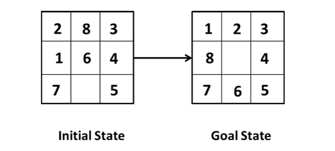(An example of the 8-puzzle)

The Search Begins: Finding a Solution

Problem-solving via state space search can be viewed as finding a path in a graph. This graph, often a tree, consists of:

Nodes: Data structures representing states, including parent node, action taken to reach it, path cost, and depth.
Arcs (Edges): Represent operators/actions, associated with a path cost.

The process involves:

Expansion: Generating all successor nodes of an already-explored state and adding them to the graph.
Goal Test: Checking if a newly generated node is a goal state.

A solution is a sequence of operators (actions) corresponding to a path from the start node to a goal node.

General Tree Search Algorithm

The basic idea of a tree search algorithm is an offline, simulated exploration of the state space. It typically involves maintaining a fringe (or frontier) of unexpanded nodes and iteratively picking a node from the fringe, checking if it's a goal, and if not, expanding it by generating its successors.

function TREE-SEARCH(problem) returns a solution, or failure
    initialize the fringe using the initial state of problem
    loop do
        if the fringe is empty then return failure
        node ← REMOVE-FRONT(fringe)
        if GOAL-TEST(problem, STATE(node)) then return SOLUTION(node)
        add EXPAND(node, problem) to the fringe

(A general tree search algorithm )

Evaluating Search Strategies

How do we know if a search strategy is any good? We evaluate them based on several criteria:

Completeness: Does it always find a solution if one exists?
Time Complexity: How many nodes are generated/expanded?
Space Complexity: What is the maximum number of nodes stored in memory?
Optimality: Does it always find a least-cost solution (if costs are a factor)?

These complexities are often measured in terms of:

b: The branching factor (maximum number of successors of any state).
d: The depth of the shallowest goal node (least-cost solution).
m: The maximum depth of the state space (which can be infinite).

Uninformed Search Strategies: Searching Blindfolded (But Systematically!)

Uninformed search strategies, also known as blind search, use no information about the problem other than its definition. They can only generate successors and distinguish a goal state from a non-goal state. Let's explore some common ones:

1. Breadth-First Search (BFS)

BFS explores the search tree level by level. It expands the root node first, then all successors of the root, then their successors, and so on. Think of it as ripples expanding on a pond.

Implementation: Uses a First-In, First-Out (FIFO) queue for the fringe. New successors are added to the tail of the queue.
Algorithm Sketch:
1. Initialize NODE-LIST (FIFO queue) with the initial state.
2. Loop until goal found or NODE-LIST is empty:
  - If NODE-LIST is empty, quit (failure).
  - Else, remove the first element (V) from NODE-LIST.
  - For each rule applicable to V:
    - Generate new state.
    - If goal, return state and quit.
    - Else, add new state to the end of NODE-LIST.
Properties:
- Complete? Yes (if b is finite).
- Time? $O(b^d)$ (1 + b + $b^2$ + ... + $b^d$ ).
- Space? $O(b^d)$ (keeps every node in memory, which is a major drawback).
- Optimal? Yes (if path cost is 1 per step, or more generally, a non-decreasing function of depth).

2. Uniform-Cost Search (UCS)

While BFS is optimal for equal step costs, UCS generalizes this by always expanding the node n with the lowest path cost g(n) (cost from start to n). It cares about the total cost, not just the number of steps.

Implementation: Uses a priority queue for the fringe, ordered by path cost g(n).
Properties:
- Complete? Yes, if the cost of every step is $\ge \epsilon$ (a small positive constant) to avoid infinite loops with zero-cost actions (like a NoOp).
- Time? $O(b^{\lceil C*/\epsilon \rceil})$ , where $C^*$ is the cost of the optimal solution. Can be much larger than $b^d$ .
- Space? $O(b^{\lceil C*/\epsilon \rceil})$ .
- Optimal? Yes, because nodes are expanded in increasing order of g(n).

3. Depth-First Search (DFS)

DFS always expands the deepest unexpanded node in the current fringe of the search tree. It explores one branch of the tree as far as possible before backtracking.

Implementation: Uses a Last-In, First-Out (LIFO) queue (a stack) for the fringe. Successors are added to the front.
Algorithm Sketch:
1. Form a stack with the root node.
2. Loop until stack is empty or goal found:
  - Remove the top element. If goal, success.
  - Else, add its children to the top of the stack.
Properties:
- Complete? No. It can fail in infinite-depth spaces or get stuck in loops. (It's complete for finite spaces if modified to avoid repeated states along a path ).
- Time? $O(b^m)$ , where m is the maximum depth. Terrible if m is much larger than d, but can be faster than BFS if solutions are dense and deep.
- Space? $O(bm)$ (linear space!), as it only needs to store a single path from the root to a leaf node, along with the unexpanded sibling nodes for each node on the path.
- Optimal? No. It might find a suboptimal solution by going down a very long path.

4. Depth-Limited Search (DLS)

To address DFS's problem of getting lost in infinite branches, DLS imposes a depth limit l. Nodes at depth l are treated as if they have no successors.

Choosing l: Critical. Too deep is wasteful; too shallow ( $l < d$ ) means it won't find a solution.
Properties:
- Complete? Yes, if $l \ge d$ .
- Time? $O(b^l)$ .
- Space? $O(bl)$ (linear space).
- Optimal? No.

5. Iterative Deepening Search (IDS)

IDS combines the benefits of BFS and DFS. It repeatedly applies DLS with increasing depth limits: 0, 1, 2, ..., until a solution is found.

Overhead: While it seems wasteful to re-expand nodes, the overhead is often small compared to the exponential growth of the search tree, especially for large branching factors. For example, with b=10, d=5, the overhead is about 11%.
Properties:
- Complete? Yes (like BFS, if b is finite).
- Time? $O(b^d)$ .
- Space? $O(bd)$ (like DFS, linear space).
- Optimal? Yes (like BFS, if path cost is a non-decreasing function of depth).
Generally preferred for large search spaces where the solution depth is unknown.

Here's a quick summary table:

Criterion	Breadth-First	Uniform-Cost	Depth-First	Depth-Limited	Iterative Deepening
Complete?	Yes¹	Yes¹ᐟ²	No	If $l \ge d$	Yes¹
Time	$O(b^d)$	$O(b^{\lceil C*/\epsilon \rceil})$	$O(b^m)$	$O(b^l)$	$O(b^d)$
Space	$O(b^d)$	$O(b^{\lceil C*/\epsilon \rceil})$	$O(bm)$	$O(bl)$	$O(bd)$
Optimal?	Yes³	Yes	No	No	Yes³
¹ if b is finite
² if step costs $\ge \epsilon > 0$
³ if path cost is a non-decreasing function of depth

Dealing with Repeated States

A significant issue in search is repeated states, where the same state can be reached through multiple paths. Failing to detect these can turn a linear problem into an exponential one. We can implement graph search instead of tree search, which keeps track of explored states to avoid redundant work. Methods to control repeated states include:

Don't generate a node that is the same as its parent.
Don't create paths with cycles (check ancestors).
Don't generate any state that has been generated before (requires storing all explored states, $O(b^d)$ space).

Informed Search Strategies: Searching with a Guide ️

Uninformed search is often inefficient. Informed (or heuristic) search strategies use problem-specific knowledge beyond the problem definition itself to guide the search more efficiently. They identify whether one non-goal state is "more promising" than another.

Heuristic Functions: The Agent's Compass

The core of informed search is the heuristic function, denoted as $h(n)$ .

$h(n)$ = estimated cost of the cheapest path from the state at node n to a goal state.

It's an estimate of "desirability" – how close a state is to the goal. Finding a good heuristic is key but not always easy.

1. Hill-Climbing Search (Local Search)

Hill-climbing is a local search algorithm that continuously moves in the direction of increasing value (uphill). It doesn't maintain a full search tree, only the current state and its objective function value. It doesn't look ahead beyond the immediate neighbors.

Algorithm (Basic):
1. Evaluate initial state. If goal, return. Else, current state = initial state.
2. Loop until solution or no new operators:
  - Select an untried operator, apply to current state to get new state.
  - Evaluate new state: If goal, return. If better than current, new state becomes current. Else, continue loop.
Steepest-Ascent Hill Climbing: Considers all moves from the current state and selects the best one as the next state.
Problems:
- Local Maxima: A state better than all neighbors but not the global optimum. Solution: random restart or backtracking.
- Plateaus: A flat area where neighbors have the same value. Solution: expand a few generations ahead.
- Ridges: Areas higher than surroundings but with slopes that make single-move traversal impossible. Solution: apply several operators before evaluation.
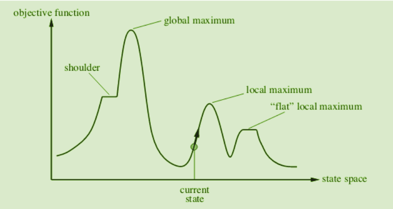(Visual representation of local maximum, plateau, and ridge)

2. Best-First Search

This is a general approach where a node is selected for expansion based on an evaluation function $f(n)$ . The node with the "most desirable" $f(n)$ is chosen.

Implementation: Uses a priority queue (OPEN list) for the fringe, ordered by $f(n)$ . A CLOSED list keeps track of expanded nodes.

3. Greedy Best-First Search

A specific type of best-first search where the evaluation function is just the heuristic function: $f(n) = h(n)$ . It tries to expand the node that appears to be closest to the goal.

It follows a single path but can switch if another appears more promising.
Example: Using straight-line distance (SLD) as $h(n)$ for route finding.
Properties:
- Complete? No. Can get stuck in loops.
- Time? $O(b^m)$ in worst case, but a good heuristic can give dramatic improvement.
- Space? $O(b^m)$ (keeps all nodes in memory).
- Optimal? No.

4. A* Search: The Star of the Show

A* search is a best-first search that aims to find the least-cost path. It evaluates nodes by combining $g(n)$ (the cost to reach the node) and $h(n)$ (the estimated cost to get from the node to the goal): $f(n) = g(n) + h(n)$ This $f(n)$ is the estimated total cost of the cheapest solution path through node $n$ .

Algorithm Sketch (simplified from ):
1. Start with OPEN list containing only the initial node ( $g=0, f=h$ ). CLOSED list is empty.
2. Loop until goal found or OPEN is empty:
  - If OPEN empty, fail.
  - Pick node from OPEN with lowest $f$ value (BESTNODE). Move to CLOSED.
  - If BESTNODE is goal, return solution.
  - Else, generate successors. For each successor:
    - Calculate $g(\text{successor}) = g(\text{BESTNODE}) + \text{cost(BESTNODE, successor)}$ .
    - If successor is on OPEN or CLOSED with a worse $g$ value, update its parent, $g$ , and $f$ .
    - If successor not on OPEN or CLOSED, add to OPEN, calculate $f(\text{successor})$ .
Properties:
- Complete? Yes (unless there are infinitely many nodes with $f \le f(G)$ ).
- Time? Exponential in the worst case.
- Space? Keeps all nodes in memory (can be an issue).
- Optimal? Yes, if the heuristic $h(n)$ is admissible (for tree search) or consistent (for graph search).

Admissible Heuristics: A heuristic $h(n)$ is admissible if it never overestimates the true cost to reach the goal from $n$ (i.e., $h(n) \le h^*(n)$ ). It's optimistic! Example: straight-line distance for route finding. A* using TREE-SEARCH is optimal if $h(n)$ is admissible.

Consistent Heuristics (Monotonicity): A heuristic is consistent if for every node $n$ and every successor $n'$ of $n$ generated by action $a$ , $h(n) \le \text{cost}(n, a, n') + h(n')$ . This means the $f$ -cost along any path is non-decreasing. Consistency implies admissibility. A* using GRAPH-SEARCH is optimal if $h(n)$ is consistent.

Relaxed Problems: A good way to create admissible heuristics is to solve a "relaxed" version of the problem (one with fewer restrictions on actions). The cost of an optimal solution to a relaxed problem is an admissible heuristic for the original problem. For the 8-puzzle, examples include $h_1(n)$ = number of misplaced tiles and $h_2(n)$ = sum of Manhattan distances of tiles to their goal positions. Both are admissible.

Online Search Agents and Unknown Environments

So far, we've mostly discussed offline search, where the agent computes a complete solution before taking any action. But what if the environment is unknown, or changes dynamically? This is where online search agents come in.

These agents operate by interleaving computation and action. They take an action, then observe the environment and compute the next action. This is crucial for:

Unknown environments: Where the agent doesn't know the full state space or the effects of its actions beforehand. It has to learn as it goes.
Partially observable environments: Where the agent cannot sense the entire state of the world.
Dynamic environments: Where the world can change independently of the agent's actions.

Learning agents are a type of online agent that explicitly improve their performance with experience. They can adapt their strategies based on what they discover about the environment. For example, a robot exploring an unknown planet would use online search, learning the terrain and potential hazards as it moves.

The strategies for online search often involve exploration (to discover new parts of the state space) and exploitation (to use known paths to reach goals). The agent might need to make decisions with incomplete information, balancing the risk of taking a "wrong" step with the need to gather more information.

Conclusion: The Art of Navigating Complexity

Solving problems through searching is a fundamental AI paradigm. We've seen how problems are formally defined and how different strategies can be employed:

Uninformed searches like BFS, DFS, and IDS provide systematic ways to explore, with IDS often being a good general-purpose choice when solution depth is unknown.
Informed searches like Greedy Best-First and A* use heuristic functions to guide the search more intelligently, with A* guaranteeing optimality if its heuristic is well-chosen (admissible/consistent).
Online search agents tackle the challenge of unknown or dynamic environments by interleaving action and planning.

The choice of search strategy depends heavily on the problem's nature, the availability of good heuristics, and constraints on time and memory. The journey from a problem statement to a solution is a fascinating exploration of logic, strategy, and computational power!