P, NP, and Beyond - A Guide to Understanding Computational Complexity Classes

Hey everyone, and welcome back to the blog! When we design algorithms to solve problems, we're often concerned with how efficient they are. But have you ever wondered about the inherent difficulty of the problems themselves? Can all problems be solved quickly by computers, or are some fundamentally "harder" than others? This is where the fascinating field of Computational Complexity Theory comes in, and at its heart are Complexity Classes.

These classes help us categorize problems based on the computational resources (like time or memory) required to solve them. Understanding these classes, especially P, NP, NP-Complete, and NP-Hard, provides a framework for grasping the limits of computation and the relationships between different types of challenging problems. It's a topic that resonates deeply in theoretical computer science and has practical implications for us developers.

What are Complexity Classes? Sorting Problems by Difficulty

Complexity Classes are sets that categorize computational problems based on their resource requirements. The main goal is to classify problems according to how much computational effort (typically time or space) is needed to solve them, usually as a function of the input size. This provides a way to understand the inherent difficulty of a problem and how it relates to other problems.

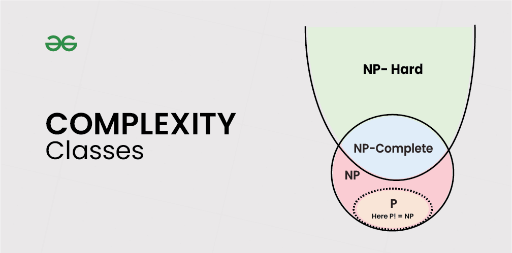
The image you might have seen (often depicted as a Venn diagram with P inside NP, and NP-Complete as the hard core of NP) helps visualize some of these relationships.

Key Types of Complexity Classes

Let's explore some of the most well-known complexity classes:

Class P: The "Efficiently Solvable" Problems

• Definition: The class P (Polynomial time) contains all decision problems that can be solved by a deterministic Turing machine in polynomial time.
  • A decision problem is a problem with a yes/no answer (e.g., "Is this number prime?" or "Does this graph have a path from A to B?").
  • A deterministic Turing machine is a theoretical model of computation that can simulate any algorithm that runs on a classical computer. Essentially, it means the algorithm has no randomness and follows a fixed set of steps.
  • Polynomial time means the number of computational steps required by the algorithm is bounded by a polynomial function of the input size $n$ (e.g., O(n), O(n²), O(n³)).
• Significance: Problems in P are generally considered "tractable" or "efficiently solvable" by computers. Many practical problems we encounter daily fall into this class (e.g., sorting an array, searching in a sorted array, finding the shortest path in a graph using Dijkstra's algorithm).

Class NP: The "Efficiently Verifiable" Problems

• Definition: The class NP (Nondeterministic Polynomial time) contains all decision problems for which a given proposed solution (a "certificate" or "witness") can be verified as correct in polynomial time by a deterministic Turing machine.
• Explanation: This means if someone gives you a potential "yes" answer and a proof (certificate), you can check if that proof is valid for the problem in polynomial time. It doesn't mean you can find the solution in polynomial time, just that you can check a proposed one quickly.
  • An alternative definition is that NP problems are those solvable in polynomial time by a nondeterministic Turing machine (a theoretical machine that can "guess" a solution and then verify it).
• Significance: NP is a very famous and important complexity class. It contains many critical problems in computer science and mathematics, including some that we don't know how to solve efficiently (like the Traveling Salesman Problem or the Boolean Satisfiability Problem - SAT).
• Relationship to P: All problems in P are also in NP (P ⊆ NP). If a problem can be solved in polynomial time, then a given solution can certainly be verified in polynomial time (by simply solving it again and comparing).

Class NP-Complete: The Hardest Problems in NP

• Definition: A decision problem is NP-Complete if it satisfies two conditions:
  1. It is in the class NP (i.e., a given solution can be verified in polynomial time).
  2. It is NP-hard (meaning every other problem in NP can be reduced to it in polynomial time – more on NP-hard below).
• Significance: NP-Complete problems are, in a sense, the "hardest" problems in NP. If you could find an efficient (polynomial-time) algorithm for any single NP-Complete problem, then you would have found an efficient algorithm for all problems in NP (due to the reducibility property). This would mean P = NP!
• Examples: The Traveling Salesman Problem (decision version), Boolean Satisfiability Problem (SAT), Vertex Cover, Hamiltonian Cycle problem, Graph Coloring (decision version).
• Discovery: The concept of NP-completeness was developed by Stephen Cook and Leonid Levin in the early 1970s (Cook-Levin theorem, which proved SAT is NP-Complete). Richard Karp later showed many other problems were NP-Complete by reducing SAT to them.

Class NP-Hard: At Least as Hard as NP-Complete

• Definition: A problem is NP-Hard if every problem in NP can be reduced to it in polynomial time. This means an NP-Hard problem is at least as hard as any problem in NP.
• Key Difference from NP-Complete: An NP-Hard problem does not necessarily have to be in NP itself. It might not even be a decision problem (it could be an optimization problem, like finding the shortest TSP tour, not just deciding if a tour of a certain length exists). If an NP-Hard problem is also in NP, then it is NP-Complete.
• Significance: NP-Hard problems are also considered inherently difficult to solve efficiently. Finding a polynomial-time algorithm for an NP-Hard problem would imply P = NP (if the problem is a decision problem also in NP) or would solve all NP problems efficiently.
• Examples: The optimization version of the Traveling Salesman Problem, the Halting Problem (which is undecidable, thus much harder than NP-Complete).

Key Complexity Relationships

Understanding how these classes relate to each other is crucial:

P vs. NP: The Million-Dollar Question

• This is the most famous unsolved problem in theoretical computer science (and one of the Clay Mathematics Institute's Millennium Prize Problems).
• It asks: Is P equal to NP? In other words, if a solution to a problem can be verified quickly (in polynomial time), can the solution itself also be found quickly (in polynomial time)?
  • If P = NP, then many currently intractable problems (like those in NP-Complete) could be solved efficiently. This would have profound implications for fields like cryptography, optimization, AI, and more.
  • If P ≠ NP (which is what most computer scientists believe), then there are problems in NP that are inherently difficult to solve, meaning no polynomial-time algorithm exists for them.
• The consensus is that P ≠ NP, but a formal proof is still elusive.

NP-Complete vs. NP-Hard

• Every NP-Complete problem is also NP-Hard. This is by definition, as NP-Complete problems must be in NP and be NP-Hard.
• However, not every NP-Hard problem is NP-Complete. An NP-Hard problem might not be a decision problem, or it might not be in NP (i.e., a solution cannot be verified in polynomial time). For example, the Halting Problem is NP-Hard but not in NP (it's undecidable).
• NP-Complete problems are essentially the "hardest problems within NP."

The study of these complexity classes has led to many breakthroughs in our understanding of algorithms and the limits of computation.

Why Does This Matter for Developers?

While these concepts are rooted in theoretical computer science, they have practical implications:

• Problem Recognition: If you identify that a problem you're trying to solve is NP-Complete, you know that finding an efficient, exact algorithm is likely impossible (assuming P ≠ NP). This can save you from a fruitless search for a "perfect" fast solution.
• Strategy Shift: For NP-Complete/NP-Hard problems, developers often turn to:
  • Approximation Algorithms: Find a solution that is close to optimal in polynomial time.
  • Heuristic Algorithms: Use rules of thumb or educated guesses to find good solutions quickly, without guarantees of optimality (e.g., greedy algorithms for some problems, local search).
  • Randomized Algorithms: Use randomness to find solutions with high probability.
  • Solving for Special Cases: The problem might be solvable in polynomial time for specific constraints or smaller instances.
  • Fixed-Parameter Tractable Algorithms: If some parameter of the problem is small, it might be solvable efficiently.
• Setting Expectations: Understanding problem complexity helps in setting realistic expectations for performance and solution quality.

Key Takeaways

• Complexity Classes (like P, NP, NP-Complete, NP-Hard) categorize computational problems based on the resources needed to solve them.
• P problems are solvable efficiently (polynomial time) by a deterministic machine.
• NP problems have solutions that can be verified efficiently (polynomial time).
• NP-Complete problems are the hardest problems in NP; if one can be solved efficiently, all can.
• NP-Hard problems are at least as hard as any NP problem.
• The P vs. NP problem remains a major open question in computer science, with most believing P ≠ NP.
• Recognizing the complexity class of a problem guides the choice of algorithmic strategies.

While wrestling with P vs. NP might not be part of our daily coding tasks, being aware of these concepts helps us appreciate the deeper underpinnings of the computational challenges we face and guides us toward more pragmatic and effective solutions for hard problems.