Magnetism Unveiled - The Universe's Invisible & Attractive Force!

February 10, 2023 — #Physics #Electromagnetism

Hey there, curious comrades and field explorers! Ever been utterly baffled by how a simple magnet can stick to your fridge, defying gravity without any visible strings attached? Or how a compass magically points north, guiding travelers for centuries? And let's not forget those futuristic MRI machines that see inside our bodies! What's the invisible wizardry behind all this? It's Magnetism, one of the most fascinating and fundamental forces shaping our universe!

This isn't just about kids' toys; magnetism is a powerhouse. It's born from the motion of electric charges and creates invisible magnetic fields that can push, pull, and make charged particles dance in intricate patterns. From the microscopic jiggle of electrons to the Earth's own protective magnetic bubble, this force is an unsung hero.

So, if you've ever wondered why magnets seem to have an inexhaustible supply of "stickiness," how they can generate electricity, or what makes some materials magnetic while others are utterly indifferent, you're in for a treat! We're going on an electrifying (and magnetizing!) journey to unpack the secrets of this pervasive force. Let’s dive in—it’s bound to be attractive!

The Fundamental Attraction: What IS Magnetic Force?

Magnetism all starts with force – the push or pull that magnetic objects or moving charges exert on each other.

An Old View: Coulomb's Law for Magnetic Poles (A Historical Nod)

Historically, magnetism was often described in terms of "magnetic poles" (North and South), similar to electric charges. An early attempt to quantify the force between two hypothetical magnetic poles ( $m_1$ and $m_2$ ) separated by a distance $r$ was given by a law analogous to Coulomb's law for electric charges: $F = k \frac{m_1 m_2}{r^2} = \frac{\mu_0}{4\pi} \frac{m_1 m_2}{r^2}$ Where $F$ is the force, and $k = \mu_0/(4\pi)$ is the proportionality constant, with $\mu_0$ being the permeability of free space. Important Note: While this "pole" concept can be useful for visualizing simple bar magnets, modern physics understands magnetism as fundamentally arising from moving electric charges and intrinsic magnetic moments (like electron spin), not isolated magnetic monopoles (which, as far as we know, don't exist!).

The Real Deal: Lorentz Force on Moving Charges! ️

The true heart of magnetic force on a charge is captured by the Lorentz force law. It states that a charge $q$ moving with velocity $\vec{v}$ in a magnetic field $\vec{B}$ experiences a magnetic force $\vec{F}_m$ : $\vec{F}_m = q(\vec{v} \times \vec{B})$ The magnitude of this force is $F_m = qvB\sin\theta$ , where $\theta$ is the angle between $\vec{v}$ and $\vec{B}$ . Key things about this force:

It only acts on moving charges. No motion, no magnetic force!
The force is always perpendicular to both the velocity $\vec{v}$ AND the magnetic field $\vec{B}$ (its direction is given by the right-hand rule).
Because the force is always perpendicular to the velocity, magnetic forces do no work on isolated charges (they can change direction, but not speed/kinetic energy).

Charged Particles Gone Wild: Dancing in Magnetic Fields!

What happens when a charged particle finds itself zipping through a magnetic field? Thanks to the Lorentz force, it gets taken for a wild ride!

If a charged particle $q$ with mass $m$ enters a uniform magnetic field $\vec{B}$ with a velocity component $\vec{v}_\perp$ perpendicular to $\vec{B}$ , the magnetic force $F_m = qv_\perp B$ acts as a centripetal force, causing the particle to move in a circular path.

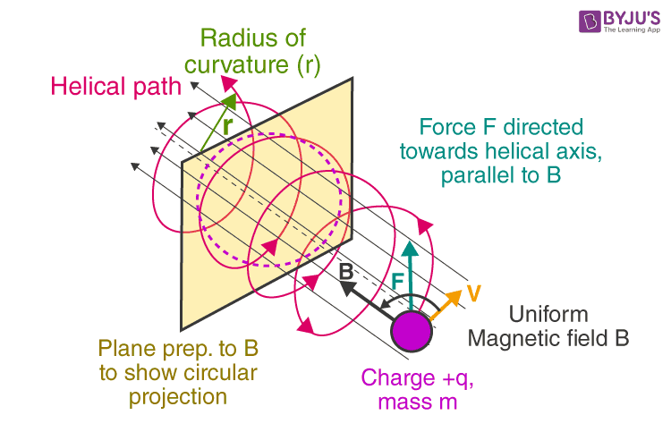Motion of a charged particle in a magnetic field, showing helical path (Image: A charged particle entering a magnetic field at an angle traces a helical path.)

If the initial velocity $\vec{v}$ has a component $v_\parallel$ parallel to $\vec{B}$ and a component $v_\perp$ perpendicular to $\vec{B}$ (so $\vec{v}$ is at an angle $\theta$ to $\vec{B}$ , with $v_\perp = v\sin\theta$ and $v_\parallel = v\cos\theta$ ):

The perpendicular component $v_\perp$ leads to circular motion.
The parallel component $v_\parallel$ is unaffected by $\vec{B}$ (since $\vec{v}_\parallel \times \vec{B} = 0$ ), so the particle continues to drift along the field lines.

The combination results in a helical (spiral) path.

Let's break down the circular part of the motion (due to $v_\perp = v\sin\theta$ ): The magnetic force provides the centripetal force: $q (v\sin\theta) B = \frac{m (v\sin\theta)^2}{R}$ Where $R$ is the radius of the circular component of the path. Solving for $R$ : $R = \frac{m(v\sin\theta)}{qB} = \frac{mv_\perp}{qB}$ The angular frequency ( $\omega$ ) of this circular motion (also called cyclotron frequency) is: $\omega = \frac{v_\perp}{R} = \frac{v\sin\theta}{mv\sin\theta / (qB)} = \frac{qB}{m}$ Notice $\omega$ doesn't depend on $v$ or $\theta$ (for the circular part)! The time period ( $T$ ) for one revolution is: $T = \frac{2\pi}{\omega} = \frac{2\pi m}{qB}$ The pitch of the helix (distance moved along the field line in one revolution) is $p = v_\parallel T = (v\cos\theta) \frac{2\pi m}{qB}$ .

Equations of Motion for a Helical Path: If $\vec{B}$ is along the x-axis ( $B_x = B, B_y=B_z=0$ ) and the particle's velocity at $t=0$ is in the x-y plane, $\vec{v}_0 = v_0(\cos\alpha \hat{i} + \sin\alpha \hat{j})$ (where $\alpha$ here is the angle velocity makes with B-field, previously $\theta$ ). Let's use a setup where $\vec{B}$ is along x-axis, and $\vec{v} = v (\cos \theta \hat{i} + \sin \theta \hat{j})$ . The circular motion will be in the y-z plane, with radius $R = \frac{mv\sin\theta}{qB}$ and angular frequency $\omega = \frac{qB}{m}$ . The particle's position $(r_x, r_y, r_z)$ at time $t$ , assuming it starts at the origin:

Motion along the field (x-axis): $r_x(t) = (v\cos\theta) t$
Circular motion in the y-z plane (radius $R$ ): If we set the phase such that at $t=0$ , $v_y(0)=v\sin\theta$ (used to determine $R$ ) and then the circle starts: $r_y(t) = R \sin(\omega t) = \frac{mv\sin\theta}{qB} \sin\left(\frac{qB}{m}t\right)$ $r_z(t) = R(1 - \cos(\omega t)) = \frac{mv\sin\theta}{qB} \left(1 - \cos\left(\frac{qB}{m}t\right)\right)$
Case 1: $\theta = 0$ (velocity parallel to $\vec{B}$ ) $\sin\theta = 0$ , so $F_m = 0$ . The particle moves in a straight line: $r_x = vt$ , $r_y=0$ , $r_z=0$ . No drama!
Case 2: $\theta = \pi/2$ (velocity perpendicular to $\vec{B}$ ) $\cos\theta = 0, \sin\theta = 1$ . So $r_x = 0$ . The motion is a perfect circle in the y-z plane with radius $R = mv/(qB)$ . $r_y(t) = R \sin(\omega t)$ , $r_z(t) = R(1 - \cos(\omega t))$ .

The Ultimate Electrified Tango: Charges in Combined E and B Fields!

What if a poor charged particle has to deal with both an electric field $\vec{E}$ AND a magnetic field $\vec{B}$ ? The total force is the sum of the electric force ( $q\vec{E}$ ) and the magnetic force ( $q(\vec{v} \times \vec{B})$ ). This is the full Lorentz Force Law: $\vec{F} = q(\vec{E} + \vec{v} \times \vec{B})$ The motion can get incredibly complex, from gentle drifts to wild cycloids! Given $\vec{v} = v_x\hat{i} + v_y\hat{j} + v_z\hat{k}$ , $\vec{E} = E_x\hat{i} + E_y\hat{j} + E_z\hat{k}$ , and $\vec{B} = B_x\hat{i} + B_y\hat{j} + B_z\hat{k}$ . The force components are: $F_x = q[E_x + (v_y B_z - v_z B_y)]$ $F_y = q[E_y + (v_z B_x - v_x B_z)]$ $F_z = q[E_z + (v_x B_y - v_y B_x)]$ And the equations of motion ( $m\frac{d\vec{v}}{dt} = \vec{F}$ ) become three coupled differential equations: $\frac{dv_x}{dt} = \frac{q}{m}(E_x + v_y B_z - v_z B_y)$ $\frac{dv_y}{dt} = \frac{q}{m}(E_y + v_z B_x - v_x B_z)$ $\frac{dv_z}{dt} = \frac{q}{m}(E_z + v_x B_y - v_y B_x)$ Solving these in general is tough, but let's look at some special cases (let $\omega = qB_0/m$ where $B_0$ is a characteristic magnetic field strength).

Case 1: Crossed Fields - Velocity Selector & Cycloids! ( $\vec{v} = v_0\hat{i}$ , $\vec{E} = E_0\hat{j}$ , $\vec{B} = B_0\hat{k}$ ) Here, $\vec{E} \perp \vec{B}$ , and initial $\vec{v}_0$ is $\perp$ to both. Equations of motion: $\frac{dv_x}{dt} = \frac{q}{m}(v_y B_0) = \omega v_y(t)$ $\frac{dv_y}{dt} = \frac{q}{m}(E_0 - v_x B_0) = \omega \left(\frac{E_0}{B_0} - v_x(t)\right)$ $\frac{dv_z}{dt} = 0 \implies v_z(t) = 0 \text{ (if initially 0)}$ Solving these: With initial conditions $v_x(0)=v_0, v_y(0)=0, v_z(0)=0$ and particle starting at origin $(0,0,0)$ : $v_x(t) = \left(v_0 - \frac{E_0}{B_0}\right) \cos(\omega t) + \frac{E_0}{B_0}$ $v_y(t) = -\left(v_0 - \frac{E_0}{B_0}\right) \sin(\omega t)$ And integrating for position: $r_x(t) = \frac{E_0}{B_0}t + \frac{1}{\omega}\left(v_0 - \frac{E_0}{B_0}\right)\sin(\omega t)$ $r_y(t) = \frac{1}{\omega}\left(v_0 - \frac{E_0}{B_0}\right)(\cos(\omega t) - 1)$

Velocity Selector: If $v_0 = E_0/B_0$ , then $v_x(t) = v_0$ and $v_y(t) = 0$ . The particle moves in a straight line undeflected! This setup is used to select particles of a specific velocity.
Cycloidal Motion: If $v_0 = 0$ (starts from rest): $r_x(t) = \frac{E_0}{B_0\omega}(\omega t - \sin(\omega t))$ $r_y(t) = \frac{E_0}{B_0\omega}(1 - \cos(\omega t))$ This is the path of a point on the rim of a rolling wheel – a cycloid.

Case 2: $\vec{v}$ starts along $\vec{E}$ , both $\perp \vec{B}$ ( $\vec{v}_0 = v_0\hat{i}$ , $\vec{E} = E_0\hat{i}$ , $\vec{B} = B_0\hat{k}$ ) Equations of motion: $\frac{dv_x}{dt} = \frac{q}{m}(E_0 + v_y B_0) = \omega\left(\frac{E_0}{B_0} + v_y(t)\right)$ $\frac{dv_y}{dt} = -\frac{q}{m}(v_x B_0) = -\omega v_x(t)$ With $v_x(0)=v_0, v_y(0)=0, v_z(0)=0$ and starting at origin:

Subcase 2.1: $v_x(t) = \frac{E_0}{B_0}\sin(\omega t) + v_0\cos(\omega t)$ $v_y(t) = \frac{E_0}{B_0}(\cos(\omega t)-1) - v_0\sin(\omega t)$ Positions: $r_x(t) = \frac{E_0}{B_0\omega}(1-\cos(\omega t)) + \frac{v_0}{\omega}\sin(\omega t)$ $r_y(t) = \frac{E_0}{B_0\omega}(\sin(\omega t)-\omega t) - \frac{v_0}{\omega}(1-\cos(\omega t))$
Subcase 2.2 (This assumes $v_x$ has a constant part $v_0$ and an oscillatory part): $v_x(t) = \frac{E_0}{B_0}\sin(\omega t) + v_0$ $v_y(t) = \frac{E_0}{B_0}(\cos(\omega t)-1)$ Positions: $r_x(t) = \frac{E_0}{B_0\omega}(1-\cos(\omega t)) + v_0 t$ $r_y(t) = \frac{E_0}{B_0\omega}(\sin(\omega t)-\omega t)$ If $v_0=0$ (starts from rest), both subcases yield the same cycloid-like path (though different from Case 1's cycloid orientation due to $\vec{E}$ direction).

Case 3: $\vec{v}_0 \perp \vec{E} \parallel \vec{B}$ ( $\vec{v}_0=v_0\hat{i}$ , $\vec{E}=E_0\hat{j}$ , $\vec{B}=B_0\hat{j}$ ) Electric field and magnetic field are parallel. Equations of motion: $\frac{dv_x}{dt} = -\frac{q}{m}(v_z B_0) = -\omega v_z(t)$ $\frac{dv_y}{dt} = \frac{q}{m}E_0 \text{ (constant acceleration along y)}$ $\frac{dv_z}{dt} = \frac{q}{m}(v_x B_0) = \omega v_x(t)$ With $v_x(0)=v_0, v_y(0)=0, v_z(0)=0$ and starting at origin: $v_x(t) = v_0 \cos(\omega t)$ $v_y(t) = \left(\frac{qE_0}{m}\right)t$ $v_z(t) = v_0 \sin(\omega t)$ Positions: $r_x(t) = \frac{v_0}{\omega}\sin(\omega t)$ $r_y(t) = \frac{1}{2}\left(\frac{qE_0}{m}\right)t^2$ $r_z(t) = \frac{v_0}{\omega}(1-\cos(\omega t))$ This describes helical motion in the x-z plane (due to $\vec{B}$ ) combined with constant acceleration in the y-direction (due to $\vec{E}$ ). If $v_0=0$ , it's just straight-line accelerated motion along $\vec{E}$ .

Case 4: $\vec{v}_0 \parallel \vec{B} \perp \vec{E}$ ( $\vec{v}_0=v_0\hat{i}$ , $\vec{E}=E_0\hat{j}$ , $\vec{B}=B_0\hat{i}$ ) Magnetic field is parallel to initial velocity. Equations of motion: $\frac{dv_x}{dt} = 0 \implies v_x(t) = v_0$ $\frac{dv_y}{dt} = \frac{q}{m}(E_0 + v_z B_0) = \omega\left(\frac{E_0}{B_0} + v_z(t)\right)$ $\frac{dv_z}{dt} = -\frac{q}{m}(v_y B_0) = -\omega v_y(t)$ This is similar to Case 2's equations for $v_y, v_z$ (with roles of $v_x, v_y$ swapped for $v_y, v_z$ ). With $v_x(0)=v_0, v_y(0)=0, v_z(0)=0$ and starting at origin: $v_x(t) = v_0$ $v_y(t) = \frac{E_0}{B_0}\sin(\omega t)$ $v_z(t) = \frac{E_0}{B_0}(\cos(\omega t)-1)$ Positions: $r_x(t) = v_0 t$ $r_y(t) = \frac{E_0}{B_0\omega}(1-\cos(\omega t))$ $r_z(t) = \frac{E_0}{B_0\omega}(\sin(\omega t)-\omega t)$ This is a drift along x (due to initial $v_0$ since $\vec{B}$ is along x) combined with cycloidal motion in the y-z plane. If $v_0=0$ , it's pure cycloidal motion in y-z.

Case 5: $\vec{v}_0 \parallel \vec{E} \parallel \vec{B}$ ( $\vec{v}_0=v_0\hat{i}$ , $\vec{E}=E_0\hat{i}$ , $\vec{B}=B_0\hat{i}$ ) All three vectors are parallel! Magnetic force $\vec{v} \times \vec{B} = 0$ because $\vec{v}$ will remain parallel to $\vec{B}$ . Equations of motion: $\frac{dv_x}{dt} = \frac{q}{m}E_0 \text{ (constant acceleration along x)}$ $\frac{dv_y}{dt} = 0 \implies v_y(t)=0$ $\frac{dv_z}{dt} = 0 \implies v_z(t)=0$ With $v_x(0)=v_0, v_y(0)=0, v_z(0)=0$ and starting at origin: $v_x(t) = v_0 + \left(\frac{qE_0}{m}\right)t$ $v_y(t) = 0, \quad v_z(t) = 0$ Positions: $r_x(t) = v_0 t + \frac{1}{2}\left(\frac{qE_0}{m}\right)t^2$ $r_y(t) = 0, \quad r_z(t) = 0$ The particle simply undergoes uniformly accelerated motion along the common direction of $\vec{E}$ and $\vec{B}$ . The magnetic field has no effect!

Wires Get a Kick Too: Force on Current-Carrying Conductors!

If individual charges experience a force in a B-field, then a whole parade of charges moving as a current ( $I$ ) in a wire of length $\vec{l}$ will also feel a collective force! $\vec{F}_{wire} = I (\vec{l} \times \vec{B})$ Where $\vec{l}$ is a vector pointing along the wire in the direction of conventional current. This force is the basis for electric motors!

If the wire forms a closed loop, it can experience a torque ( $\vec{\tau}$ ) in a magnetic field. The magnetic dipole moment ( $\vec{m}$ or $\vec{\mu}$ ) of a current loop with area vector $\vec{A}$ (perpendicular to the loop, magnitude equal to area) is: $\vec{m} = I \vec{A}$ The torque on this magnetic dipole in a uniform magnetic field $\vec{B}$ is: $\vec{\tau} = \vec{m} \times \vec{B}$ This torque tries to align the loop's magnetic moment with the external field.

Mapping the Unseen: Magnetic Fields & Their Sources! ️

Magnetic fields ( $\vec{B}$ ) are vector fields permeating space, exerting forces on moving charges and magnetic materials. They're visualized by field lines that conventionally go from North to South poles outside a magnet and form closed loops.

How are these fields created by currents? The Biot-Savart Law is like Coulomb's law but for magnetism; it tells us the magnetic field $d\vec{B}$ produced by an infinitesimal current element $I d\vec{l}$ : $d\vec{B} = \frac{\mu_0}{4\pi} \frac{I (d\vec{l} \times \hat{r})}{r^2}$ Where $\mu_0$ is the permeability of free space, $d\vec{l}$ is a tiny segment of the wire carrying current $I$ , $\vec{r}$ is the position vector from $d\vec{l}$ to the point where we want to find $d\vec{B}$ , and $\hat{r}$ is the unit vector in that direction. To get the total field $\vec{B}$ from a whole wire, you integrate this expression over the wire's length.

Case Studies in B-Field Generation:

Magnetic Field due to a Straight Wire: 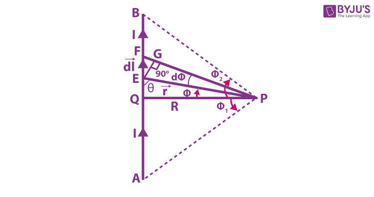(Image: Field lines are concentric circles around the wire, direction by right-hand rule.) For a straight wire segment, at a perpendicular distance $R$ from the wire, where the segment subtends angles $\phi_1$ and $\phi_2$ from the point to its ends: $B = \dfrac{\mu_0 I}{4\pi} \int \dfrac{dl \sin \theta}{r^2}$ But, $dl \sin \theta = r \sin d\phi \approx r d\phi$ and $R = r \cos \phi$ . So, $B = \dfrac{\mu_0 I}{4\pi} \int^{\phi_2}_{-\phi_1} \dfrac{d\phi}{r} = \dfrac{\mu_0 I}{4\pi} \int^{\phi_2}_{-\phi_1} \dfrac{cos \phi d\phi}{R}$ $B = \frac{\mu_0 I}{4\pi R}(\sin\phi_1 + \sin\phi_2)$ For an infinitely long straight wire: $\phi_1 = \phi_2 = \pi/2$ , so $\sin\phi_1 + \sin\phi_2 = 2$ . $B_{infinite} = \frac{\mu_0 I}{2\pi R}$ For a finite wire of length $2L$ at its perpendicular bisector: $\sin\phi = \frac{L}{\sqrt{R^2+L^2}}$ . $B_{finite} = \frac{\mu_0 I}{4\pi R} \left( \frac{2L}{\sqrt{R^2+L^2}} \right) = \frac{\mu_0 I L}{2\pi R \sqrt{R^2+L^2}}$ $B = \dfrac{\mu_0 I}{2\pi R} \sin \phi$ for a finite wire, which with $\phi_1=\phi_2=\phi$ becomes $B = \dfrac{\mu_0 I}{2\pi R} \sin \phi$ . This is correct if $\phi$ represents the half-angle subtended by the wire.
Magnetic Field due to a Curved Wire Segment (Arc): For an arc of radius $R$ subtending an angle $\theta$ (in radians) at the center: $B_{arc\_center} = \frac{\mu_0 I \theta}{4\pi R}$
Magnetic Field due to a Circular Loop (on its axis): 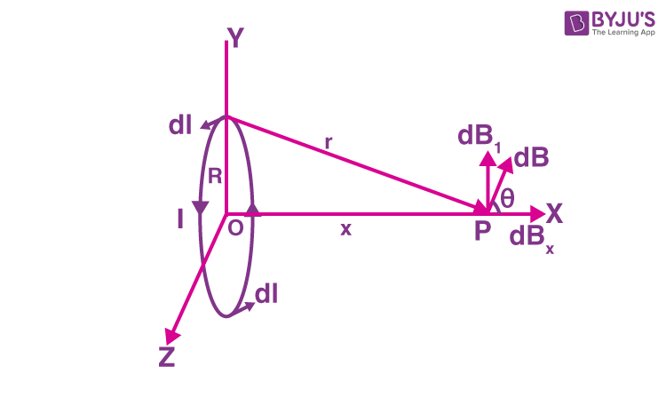(Image: Diagram showing geometry for calculating B-field on axis of a loop.) We know, $r^2 = x^2 + R^2$ and $\theta = \dfrac{\pi}{2}$ as any element of the loop will be perpendicular to the displacement vector from the element to the axial point. For a circular loop of radius $R$ carrying current $I$ , at a point $x$ along its axis from the center: $B = \dfrac{\mu_0 I}{4\pi} \int \dfrac{dl}{r^2} = \dfrac{\mu_0 I}{4\pi} \int \dfrac{dl}{x^2 + R^2}$ A null result is obtained when the components perpendicular to the x-axis are summed over, and they cancel out. The $dB_⊥$ component due to $dl$ is cancelled by the contribution due to the diametrically opposite $dl$ element. Hence, only the x-component survives. The net contribution along the x-direction can be obtained by integrating $dB_x = dB\cos\theta$ over the loop. Therefore, $B = \dfrac{\mu_0 I}{4\pi} \int \dfrac{dl}{(x^2 + R^2)} \dfrac{R}{\sqrt{x^2+R^2}} = \dfrac{\mu_0IR * 2 \pi R}{4\pi(x^2+R^2)^{\frac{3}{2}}} = \dfrac{\mu_0IR^2}{2(x^2+R^2)^{\frac{3}{2}}}$ At the center of the loop, $x = 0$ and $B = \dfrac{\mu_0I}{2R}$ .
Magnetic Fields due to Other Shapes (The Quick List!):
- Cylinder (Solid, uniform current density):
  - Inside ( $r < R_{cyl}$ ): $B = \frac{\mu_0 I r}{2\pi R_{cyl}^2}$
  - Outside ( $r > R_{cyl}$ ): $B = \frac{\mu_0 I}{2\pi r}$ (like a wire at its center)
- Solenoid (long, $n$ turns per unit length): Inside (far from ends): $B \approx \mu_0 n I$ . $B = \frac{\mu_0 n I}{2}(\sin\alpha_1 + \sin\alpha_2)$ for a finite solenoid where $\alpha_1, \alpha_2$ are angles subtended by the ends. For an infinite solenoid, $\alpha_1=\pi/2, \alpha_2=\pi/2 \implies B=\mu_0nI$ .
- Toroid ( $N$ total turns, mean radius $R$ ): Inside the toroid: $B = \frac{\mu_0 N I}{2\pi R}$ . Outside is ideally zero. (We can use $n$ for turns/length along circumference, which is $N/(2\pi R)$ ).
- N-sided Polygon (at the center): (Image related to B-field of n-sided polygon). The formula would be $B = \frac{\mu_0 n I}{2\pi a} \tan(\pi/n) \sin(\pi/n)$ , where $a$ is apothem.

Magnetic Flux ( $\Phi_B$ ): How Much B-Field "Flows" Through

This is a measure of the total magnetic field passing through a given surface area $\vec{A}$ . $\Phi_B = \int_S \vec{B} \cdot d\vec{A}$ If $\vec{B}$ is uniform and perpendicular to area $A$ , then $\Phi_B = BA$ . Its unit is the Weber (Wb).

Our Big Blue Marble Magnet: Earth's Magnetic Field!

Yes, Earth itself is a giant magnet!

Origin: Believed to be generated by the geodynamo effect – complex convective motions of molten iron and nickel in Earth's outer core.
Structure: Approximately a dipole field, tilted about $10-11^\circ$ from the Earth's rotational axis. This means the magnetic North/South poles are not at the geographic poles!
Importance:
- Navigation: Allows compasses to work.
- Protection: Deflects a significant portion of harmful charged particles from the solar wind and cosmic rays (forming the magnetosphere, leading to auroras!).

Describing Earth's Field: At any point, Earth's magnetic field $\vec{B}_E$ can be described by:

Horizontal Component ( $B_H$ ): Component parallel to Earth's surface. $B_H = B_E \cos\delta$ .
Vertical Component ( $B_V$ ): Component perpendicular to Earth's surface. $B_V = B_E \sin\delta$ .
Total Intensity ( $B_E$ or $B_T$ ): $B_E = \sqrt{B_H^2 + B_V^2}$ .
Angle of Inclination or Dip ( $\delta$ ): The angle the total field vector makes with the horizontal plane. $\tan\delta = \frac{B_V}{B_H}$
Apparent Dip Angle ( $\delta'$ ): If measured in a vertical plane not aligned with the magnetic meridian (the vertical plane containing $B_H$ ), the observed dip angle $\delta'$ is related to the true dip $\delta$ and the angle $\beta$ between the magnetic meridian and the measurement plane by: $\tan\delta' = \frac{\tan\delta}{\cos\beta}$ .

Zap! The Magic of Electromagnetic Induction!

If moving charges (currents) create magnetic fields, can changing magnetic fields create currents? YES! This is electromagnetic induction, discovered by Michael Faraday and Joseph Henry.

Faraday's Law of Induction: The electromotive force (emf, $\mathcal{E}$ – essentially a voltage) induced in a closed conducting loop is proportional to the rate of change of magnetic flux ( $\Phi_B$ ) through that loop. $\mathcal{E} = -\frac{d\Phi_B}{dt}$ This is how electric generators work! Rotate a coil in a B-field (or change the B-field through a coil), the flux changes, and an emf (and thus current, if the circuit is closed) is induced.
Lenz's Law: The Cosmic Contrarian! The minus sign in Faraday's Law is super important – it represents Lenz's Law. It states: The direction of the induced emf (and thus the induced current) is such that it creates a magnetic field that opposes the change in magnetic flux that produced it. Nature abhors a change in flux and tries to fight it! This ensures energy conservation.
Self-Inductance ( $L$ ): When the current in a coil changes, the magnetic flux it produces through itself changes. This induces a "back emf" in the coil itself, opposing the original change in current. This property is self-inductance ( $L$ ). Unit: Henry (H). $\Phi_B = LI \implies \mathcal{E}_{back} = -L \frac{dI}{dt}$ .
Mutual Inductance ( $M$ ): If two coils are near each other, a changing current in coil 1 creates a changing flux through coil 2, inducing an emf in coil 2 (and vice-versa). This is mutual inductance ( $M$ ). $\Phi_{B2} = M I_1 \implies \mathcal{E}_2 = -M \frac{dI_1}{dt}$ .

Magnetic Toolkit: Instruments & Circuits That Harness the Force! ️

Understanding magnetism lets us build amazing things!

Inductors: The Current Smoothers!

An inductor is typically a coil of wire designed to have a specific inductance $L$ . It resists changes in current. The voltage across an inductor is: $V_L = L \frac{dI}{dt}$ Energy stored in the magnetic field of an inductor carrying current $I$ : $U_L = \frac{1}{2} L I^2$ Derivation: Power to build up current is $P = V_L I = (L dI/dt)I = LI dI/dt$ . Work done $dW = P dt = LI dI$ . Total work (energy stored) $U_L = \int_0^I L I' dI' = \frac{1}{2}LI^2$ .

Series and Parallel Inductors:

Series: Inductances add up (like resistors in series). $V_{total} = V_1+V_2+\ldots = L_1\frac{dI}{dt} + L_2\frac{dI}{dt} + \ldots = (L_1+L_2+\ldots)\frac{dI}{dt} = L_{eq}\frac{dI}{dt}$ . $L_{eq, series} = L_1 + L_2 + \ldots$
Parallel: Reciprocals add up (like resistors in parallel). $dI_{total}/dt = dI_1/dt + dI_2/dt + \ldots$ . Since $V_L$ is same, $V_L/L_{eq} = V_L/L_1 + V_L/L_2 + \ldots$ . $\frac{1}{L_{eq, parallel}} = \frac{1}{L_1} + \frac{1}{L_2} + \ldots$

Circuit Adventures: LR, LC, and RLC!

Combining inductors (L), capacitors (C), and resistors (R) in circuits leads to rich behavior, especially with time-varying currents!

LR Circuits (Resistor + Inductor):
- Charging (current growth with a battery $V_0$ ): KVL: $V_0 - IR - L\frac{dI}{dt} = 0$ . Solution (with $I(0)=0$ ): $I(t) = \frac{V_0}{R}(1 - e^{-(R/L)t}) = I_{final}(1 - e^{-t/\tau})$ Where $\tau = L/R$ is the time constant. Current reaches $\approx 63.2\%$ of $I_{final}$ after one time constant.
- Discharging (current decay, battery removed, circuit shorted): KVL: $-IR - L\frac{dI}{dt} = 0$ . Solution (with $I(0)=I_0$ ): $I(t) = I_0 e^{-(R/L)t} = I_0 e^{-t/\tau}$
LC Circuits (Inductor + Capacitor): The Oscillator! KVL: $-L\frac{dI}{dt} - \frac{Q}{C} = 0$ . Since $I = dQ/dt$ , then $dI/dt = d^2Q/dt^2$ . $L\frac{d^2Q}{dt^2} + \frac{1}{C}Q = 0 \implies \frac{d^2Q}{dt^2} + \frac{1}{LC}Q = 0$ This is the equation for Simple Harmonic Motion! The solution is oscillatory: Let $\omega_0 = 1/\sqrt{LC}$ (natural angular frequency). If $Q(0)=Q_0$ (initial charge) and $I(0)=0$ : $Q(t) = Q_0 \cos(\omega_0 t)$ $I(t) = \frac{dQ}{dt} = -Q_0 \omega_0 \sin(\omega_0 t)$ Energy sloshes back and forth between capacitor's E-field and inductor's B-field.
- LC circuit with a battery $V_0$ (charging a capacitor through an inductor): KVL: $V_0 - L\frac{d^2Q}{dt^2} - \frac{Q}{C} = 0 \implies L\frac{d^2Q}{dt^2} + \frac{1}{C}Q = V_0$ . Particular solution $Q_p = CV_0$ . General solution $Q(t) = A\cos(\omega_0 t) + B\sin(\omega_0 t) + CV_0$ . If $Q(0)=0, I(0)=0$ : $A = -CV_0, B=0$ . $Q(t) = CV_0 (1 - \cos(\omega_0 t))$ $I(t) = \frac{dQ}{dt} = CV_0 \omega_0 \sin(\omega_0 t) = V_0 \sqrt{C/L} \sin(\omega_0 t)$ The charge can oscillate up to $2CV_0$ !
RLC Circuits (Resistor + Inductor + Capacitor in Series): Damped Oscillations! KVL: $-IR - L\frac{dI}{dt} - \frac{Q}{C} = 0$ . $L\frac{d^2Q}{dt^2} + R\frac{dQ}{dt} + \frac{1}{C}Q = 0$ This is a damped harmonic oscillator equation! Assume solution $Q(t) = Ae^{rt}$ . Characteristic equation: $Lr^2 + Rr + 1/C = 0$ . Roots: $r = \frac{-R \pm \sqrt{R^2 - 4L/C}}{2L}$ . The behavior depends on the discriminant $D = R^2 - 4L/C$ :
1. Overdamped ( $R^2 > 4L/C$ , so $D>0$ ): Two distinct real negative roots $r_1, r_2$ . $Q(t) = c_1 e^{r_1 t} + c_2 e^{r_2 t}$ . Decays to zero without oscillation.
2. Critically Damped ( $R^2 = 4L/C$ , so $D=0$ ): One real negative root $r = -R/(2L)$ . $Q(t) = (c_1 + c_2 t)e^{-Rt/(2L)}$ . Fastest decay to zero without oscillation.
3. Underdamped ( $R^2 < 4L/C$ , so $D<0$ ): Complex conjugate roots $r = -\frac{R}{2L} \pm i\omega_d$ . Where $\omega_d = \sqrt{\frac{1}{LC} - \left(\frac{R}{2L}\right)^2}$ is the damped angular frequency. $Q(t) = e^{-Rt/(2L)} (A \cos(\omega_d t) + B \sin(\omega_d t))$ Oscillatory decay.
- RLC with a battery $V_0$ : $L\frac{d^2Q}{dt^2} + R\frac{dQ}{dt} + \frac{1}{C}Q = V_0$ . Particular solution $Q_p = CV_0$ . General solution is homogeneous solution + $CV_0$ . $Q(t) = Q_{homogeneous}(t) + CV_0$ . Constants $c_1, c_2$ (or $A,B$ ) are found from initial conditions $Q(0), I(0)$ .

Detecting the Undetectable: Magnetic Measuring Devices

Galvanometer: Detects and measures small electric currents. A coil in a B-field experiences a torque proportional to current. Torque $\tau = NIAB\sin\phi$ (where $\phi$ is angle between normal to coil and B-field; for radial fields often used, $\sin\phi \approx 1$ ). This torque is balanced by a restoring torque from a spring, $\tau_{spring} = \kappa \theta_{deflection}$ . So, $\theta_{deflection} \propto I$ .
- Current Sensitivity: $S_I = \theta/I = NAB/\kappa$ .
- Voltage Sensitivity: $S_V = \theta/V = \theta/(IR_G) = NAB/(\kappa R_G)$ (where $R_G$ is galvanometer resistance).
Magnetometer: Measures strength and/or direction of magnetic fields. One type uses the period of oscillation of a known magnet in an unknown field ( $B_H$ ): $T = 2\pi \sqrt{\frac{\mathcal{I}}{MB_H}}$ (Where $\mathcal{I}$ is moment of inertia, $M$ is magnetic moment).

Magnetic Maps: Charting the Fields ️

These maps show variations in magnetic field strength or direction over an area. Used in geology (finding mineral deposits, tectonic structures), archaeology, etc. Anomalies $\Delta B$ from a localized magnetic dipole source (like a buried object with moment $M$ ) can fall off with distance $r$ like: $\Delta B \approx \frac{\mu_0}{4\pi} \frac{2M}{r^3} \text{ (along dipole axis)}$

Transformers: Voltage Changers!

These devices use mutual induction to change AC voltages. Two coils (primary $N_p$ turns, secondary $N_s$ turns) wound on a common iron core.

Voltage Ratio: Assuming ideal transformer (no flux leakage): $\frac{V_p}{V_s} = \frac{N_p}{N_s}$
Current Ratio: For an ideal transformer (100% efficient, power in = power out): $P_p = P_s \implies V_pI_p = V_sI_s$ . $\frac{I_p}{I_s} = \frac{V_s}{V_p} = \frac{N_s}{N_p}$
Power Ratio: For an ideal transformer, $P_p = P_s$ , so the ratio is 1. $\frac{P_p}{P_s} = 1$ Step-up transformers ( $N_s > N_p$ ) increase voltage (and decrease current). Step-down ( $N_s < N_p$ ) decrease voltage (and increase current). Essential for power distribution!

Key Takeaways: Your Pocket Guide to Magnetic Marvels!

What a truly attractive field of physics! From the tiniest electron spin to the Earth's global shield, magnetism is a force to be reckoned with. Here are the magnetic main points:

Lorentz Force is Boss: Magnetic force acts on moving charges ( $\vec{F} = q(\vec{v} \times \vec{B})$ ) and current-carrying wires ( $\vec{F} = I\vec{l} \times \vec{B}$ ), always perpendicular to velocity/current and the B-field. This leads to circular or helical motion for charges, and torques on current loops.
Fields from Currents: Moving charges/currents create magnetic fields, described by the Biot-Savart Law. We can calculate B-fields for wires, loops, solenoids, etc.
Earth's Magnetism: Our planet acts like a giant bar magnet, crucial for navigation and protection. Its field has horizontal ( $B_H$ ) and vertical ( $B_V$ ) components, and a dip angle ( $\delta$ ).
Induction Power: A changing magnetic flux ( $\Phi_B$ ) induces an emf ( $\mathcal{E} = -d\Phi_B/dt$ - Faraday's & Lenz's Laws). This is the heart of generators and transformers. Inductors ( $L$ ) store energy in B-fields ( $U = \frac{1}{2}LI^2$ ) and resist current changes.
Circuit Dynamics (LR, LC, RLC): These circuits show how energy is stored and transferred between electric and magnetic fields, leading to current growth/decay (LR), oscillations (LC), or damped oscillations (RLC). The math can get intense, but the behaviors are key to electronics!
Magnetic Instruments: Galvanometers measure current via magnetic torque. Magnetometers measure B-fields. Transformers efficiently change AC voltages.
Everywhere! Magnetism powers motors, generates our electricity, enables MRI, maglev trains, and data storage. It's truly a force that shapes modern technology.

Magnetism, once a curiosity of lodestones, is now understood as a deep and fundamental aspect of electromagnetism, intricately linked with electricity. Keep exploring its mysteries, and you'll find the universe is even more wonderfully interconnected than you imagined! What magnetic phenomenon fascinates you most?