Static Electricity - Unveiling Nature's Shocking Secrets!

Hey there, charge champions and field fanatics! Ever experienced that sudden, surprising jolt when you touch a doorknob after walking across a carpet? Or watched your hair stand on end after pulling off a woolly hat on a dry day? And who hasn't marveled at the raw power of a lightning bolt splitting the sky? These are all spectacular demonstrations of static electricity, a fundamental aspect of the grand force of electromagnetism.

This isn't just about minor annoyances or grand natural displays. The principles behind static electricity – the behavior of stationary or slowly moving electric charges – are the bedrock upon which much of our understanding of physics and technology is built. We're going to explore the nature of these charges, the forces they exert, the invisible "fields" they create, and how we can harness their energy. So, prepare for a journey into a world of attraction, repulsion, and electrifying potential!

---

The Spark of It All: Meet Electric Charge!

At the heart of all electrical phenomena is electric charge. It's a fundamental property of matter, just like mass.

• Two Flavors of Charge: Electric charges come in two types: positive (+) and negative (-).
  • The rule of thumb is simple: Like charges repel, opposite charges attract! Two positive charges will push each other away, as will two negative charges. But a positive and a negative charge? They're drawn to each other like moths to a flame (or electrons to a proton!).
• Charge Quantization: It Comes in Tiny Packets! Charge isn't a continuous fluid; it comes in discrete, indivisible units. The smallest unit of free charge ever observed is the elementary charge ($e$), which is the magnitude of the charge on a single electron (negative) or proton (positive). $e \approx 1.602 \times 10^{-19} \text{ Coulombs (C)}$ The Coulomb (C) is the SI unit of electric charge. Any observable amount of charge is always an integer multiple of this elementary charge. You can't have half an electron's charge!
• Conservation of Charge: You Can't Create or Destroy Net Charge! In any closed system, the total amount of electric charge remains constant. You can move charges around, separating positive from negative, or transferring them between objects, but the net charge (positives minus negatives) doesn't change. Charge is conserved.
• Conductors, Insulators, and In-Betweeners (Semiconductors):
  • Conductors (like metals) have electrons that are loosely bound and free to move throughout the material. They allow electric charge to flow easily.
  • Insulators (like glass, rubber, or dry air) have electrons that are tightly bound to their atoms. Charge does not flow easily through them.
  • Semiconductors (like silicon and germanium) are the cool kids in between. Their ability to conduct can be dramatically changed by adding impurities or applying external fields, making them the backbone of modern electronics.
• Getting Charged Up: How Objects Gain or Lose Charge There are three main ways an object can become electrically charged (i.e., develop a net positive or negative charge):
  1. Charging by Friction (Triboelectric Effect): When two different materials are rubbed together, electrons can be transferred from one material to the other. One becomes positively charged (loses electrons), and the other becomes negatively charged (gains electrons). Think rubbing a balloon on your hair!
  2. Charging by Conduction (Contact): If a charged object touches an uncharged conductive object, some charge will flow between them, sharing the charge.
  3. Charging by Induction: If you bring a charged object near a neutral conductor (without touching), the charges within the conductor will rearrange. For example, if a positive rod is brought near a metal sphere, electrons in the sphere are attracted towards the rod, leaving the far side of thesphere positively charged. If you then ground the far side, those positive charges can escape, leaving the sphere with a net negative charge even after the rod is removed. No direct contact needed for the final charging!

---

The Force is Strong (or Repulsive!) With This One: Coulomb's Law!

How strong is that attraction or repulsion between charges? Charles-Augustin de Coulomb figured this out in the 1780s. Coulomb's Law states that the magnitude of the electrostatic force ($F$) between two point charges ($q_1$ and $q_2$) is directly proportional to the product of the magnitudes of the charges and inversely proportional to the square of the distance ($r$) between them: $F = k \frac{|q_1 q_2|}{r^2}$ Where $k$ is Coulomb's constant. In SI units: $k = \frac{1}{4\pi\epsilon_0} \approx 8.9875 \times 10^9 \text{ N}\cdot\text{m}^2/\text{C}^2$ And $\epsilon_0$ is the permittivity of free space ($\epsilon_0 \approx 8.854 \times 10^{-12} \text{ C}^2/\text{N}\cdot\text{m}^2$).

• Vector Form of Coulomb's Law: Force is a vector! If $\vec{r}_{12}$ is the vector pointing from charge $q_1$ to charge $q_2$, and $\hat{r}_{12}$ is the unit vector in that direction ($\hat{r}_{12} = \vec{r}_{12} / |\vec{r}_{12}|$), then the force $\vec{F}_{12}$ exerted by $q_1$ on $q_2$ is: $\vec{F}_{12} = k \frac{q_1 q_2}{r_{12}^2} \hat{r}_{12}$ Or, if $\vec{r}_1$ and $\vec{r}_2$ are the position vectors of $q_1$ and $q_2$: $\vec{F}_{12} = \frac{1}{4\pi\epsilon_0} \frac{q_1 q_2}{|\vec{r}_2 - \vec{r}_1|^3} (\vec{r}_2 - \vec{r}_1)$ If $q_1q_2$ is positive (like charges), the force is repulsive (in direction of $\vec{r}_2-\vec{r}_1$). If negative (opposite charges), it's attractive.

• Superposition Principle: What if you have more than two charges? The net electrostatic force on any one charge is simply the vector sum of the individual forces exerted on it by all the other charges. Each pair-wise force is calculated independently using Coulomb's Law. If charge $q_0$ experiences forces $\vec{F}_{01}, \vec{F}_{02}, \ldots, \vec{F}_{0n}$ due to charges $q_1, q_2, \ldots, q_n$: $\vec{F}_{net,0} = \sum_{i=1}^{n} \vec{F}_{0i}$

For continuous distributions of charge (like on a charged rod or sphere), we use calculus, integrating the force contributions from infinitesimal charge elements $dq$.

---

Fields of Influence: The Electric Field ($\vec{E}$)!

Instead of thinking about charges directly yanking on each other across a distance (action-at-a-distance), it's incredibly useful to think in terms of fields. A charge creates an electric field ($\vec{E}$) in the space around it. Any other charge that enters this field then experiences a force due to the field at its location.

The electric field $\vec{E}$ at a point is defined as the electrostatic force $\vec{F}$ that would be experienced by a small positive test charge $q_0$ placed at that point, divided by the magnitude of the test charge: $\vec{E} = \frac{\vec{F}}{q_0}$ The unit of electric field is Newtons per Coulomb (N/C), which is also Volts per meter (V/m).

• Electric Field of a Point Charge ($q$): Using Coulomb's Law for the force on $q_0$ due to $q$: $F = k |q q_0|/r^2$. So, the magnitude of the electric field created by a point charge $q$ at a distance $r$ is: $E = k \frac{|q|}{r^2}$ In vector form, if $q$ is at $\vec{r}_0$ and we want the field at $\vec{r}$: $\vec{E}(\vec{r}) = \frac{1}{4\pi\epsilon_0} \frac{q}{|\vec{r} - \vec{r}_0|^3} (\vec{r} - \vec{r}_0)$ The field points away from a positive source charge and towards a negative source charge.

• Electric Field Lines: These are imaginary lines drawn to help visualize electric fields.

  • The tangent to a field line at any point gives the direction of $\vec{E}$ at that point.
  • Field lines originate on positive charges and terminate on negative charges (or extend to infinity).
  • The density of field lines in a region (how close together they are) represents the strength of the electric field – closer lines mean a stronger field.
  • Field lines never cross each other.

• Superposition of Electric Fields: Just like forces, the net electric field at any point due to a group of charges is the vector sum of the electric fields produced by each individual charge. $\vec{E}_{total} = \sum_i \vec{E}_i$

• Electric Field of Continuous Charge Distributions: For charges spread out over a line, surface, or volume, we find the field by integrating the contributions $d\vec{E}$ from infinitesimal charge elements $dq$: $d\vec{E} = \frac{1}{4\pi\epsilon_0} \frac{dq}{r^2}\hat{r} \implies \vec{E} = \int d\vec{E}$ We often use charge densities:

  • Linear charge density: $\lambda = dq/dl$ (charge per unit length)
  • Surface charge density: $\sigma = dq/dA$ (charge per unit area)
  • Volume charge density: $\rho = dq/dV$ (charge per unit volume)

---

Counting Field Lines: Electric Flux ($\Phi_E$) & Gauss's Law!

Electric flux ($\Phi_E$) is a measure of the "amount" of electric field passing through a given surface. Think of it like the number of field lines piercing that surface. For a uniform electric field $\vec{E}$ passing through a flat area $\vec{A}$ (where $\vec{A}$ is a vector whose magnitude is the area and direction is normal to the surface): $\Phi_E = \vec{E} \cdot \vec{A} = EA\cos\theta$. For a general surface and non-uniform field, we integrate: $\Phi_E = \int_S \vec{E} \cdot d\vec{A}$

Gauss's Law: The Big Reveal! This incredibly powerful law (one of Maxwell's equations!) relates the electric flux through any closed surface (a "Gaussian surface") to the total net charge ($Q_{enc}$) enclosed within that surface: $\Phi_E = \oint_S \vec{E} \cdot d\vec{A} = \frac{Q_{enc}}{\epsilon_0}$ Gauss's Law is amazing because it tells us that no matter how complicated the charge distribution inside, the total "flow" of E-field out of a closed surface only depends on the net charge trapped inside!

• Applications: If a charge distribution has enough symmetry (spherical, cylindrical, planar), we can choose a clever Gaussian surface to easily calculate the electric field.

---

Electric Potential: Not Voltage, But Close! (It's Energy per Charge!)

It often takes work to move a charge in an electric field. This means charges in an E-field have electric potential energy. The electric potential ($V$) at a point is defined as the electric potential energy ($U$) per unit positive test charge ($q_0$) at that point. $V = \frac{U}{q_0}$ Potential is a scalar quantity. Its SI unit is the Volt (V), where 1 Volt = 1 Joule per Coulomb (1 V = 1 J/C). The difference in electric potential between two points is often what we call voltage.

• Potential due to a Point Charge ($q$): The potential energy of $q_0$ near $q$ is $U = kqq_0/r$. So, the potential created by $q$ is: $V = \frac{U}{q_0} = k \frac{q}{r} = \frac{1}{4\pi\epsilon_0}\frac{q}{r}$ (Assuming $V=0$ at $r=\infty$).

• Potential due to Continuous Charge Distributions: $V = \frac{1}{4\pi\epsilon_0} \int \frac{dq}{r}$

• Linking Electric Field and Potential: The electric field is related to how the potential changes in space. Specifically, $\vec{E}$ points in the direction of the steepest decrease in potential $V$. $\vec{E} = -\nabla V$ Where $\nabla V$ is the gradient of $V$. In 1D, $E_x = -dV/dx$. Conversely, the potential difference between two points A and B can be found by integrating $\vec{E}$: $V_B - V_A = -\int_A^B \vec{E} \cdot d\vec{l}$.

• Equipotential Surfaces: These are surfaces where the electric potential $V$ is constant.

  • No work is done moving a charge along an equipotential surface.
  • Electric field lines are always perpendicular to equipotential surfaces.
  • They are like contour lines on a topographical map, but for electric potential.

---

Storing Up Energy: Electric Potential Energy ($U$)!

The electric potential energy ($U$) of a system of charges is the work required to assemble that system of charges by bringing them in from infinity.

• For two point charges ($q_1, q_2$) separated by distance $r$: $U = k \frac{q_1 q_2}{r} = \frac{1}{4\pi\epsilon_0}\frac{q_1 q_2}{r}$ If charges have the same sign, $U$ is positive (work had to be done against repulsion). If opposite signs, $U$ is negative (they attracted, field did work).
• Potential Energy of a System of Multiple Charges: Sum the potential energy for every unique pair of charges in the system. For three charges $q_1, q_2, q_3$: $U_{total} = U_{12} + U_{13} + U_{23} = k\left(\frac{q_1q_2}{r_{12}} + \frac{q_1q_3}{r_{13}} + \frac{q_2q_3}{r_{23}}\right)$.
• Work Done in Moving Charges: The work done by an external agent to move a charge $q$ from a point with potential $V_A$ to a point with potential $V_B$ (without changing its kinetic energy) is: $W_{ext} = q(V_B - V_A) = q\Delta V = \Delta U$ This is the change in the charge's potential energy.

---

The Dynamic Duo: Electric Dipoles!

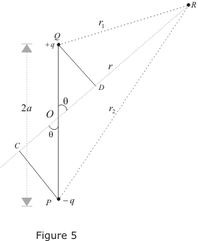
An electric dipole consists of two equal and opposite point charges, $+q$ and $-q$, separated by a small distance $d$.

• Electric Dipole Moment ($\vec{p}$): This vector quantity characterizes the dipole. $\vec{p} = q\vec{d}$ Where $\vec{d}$ is the displacement vector pointing from the negative charge to the positive charge. The magnitude is $p=qd$.

(Image: Diagram of an electric dipole, showing its field lines and equipotential surfaces.)

• Electric Potential of a Dipole (at a far point $r$, angle $\theta$ from dipole axis): Consider charges $-q$ at $z=-a$ and $+q$ at $z=+a$ (so $d=2a$, $p=2aq$). Point P at $(r, \theta)$ from origin (center of dipole). $r_1$ is distance from $+q$ to P, $r_2$ is distance from $-q$ to P. $V = \frac{q}{4\pi\epsilon_0}\left(\frac{1}{r_1} - \frac{1}{r_2}\right)$. For $r \gg a$: $r_1 \approx r - a\cos\theta$, $r_2 \approx r + a\cos\theta$. $\frac{1}{r_1} - \frac{1}{r_2} \approx \frac{1}{r(1 - (a/r)\cos\theta)} - \frac{1}{r(1 + (a/r)\cos\theta)}$ $\approx \frac{1}{r}\left( (1 + \frac{a}{r}\cos\theta) - (1 - \frac{a}{r}\cos\theta) \right)$ (using $(1\pm x)^{-1} \approx 1\mp x$) $= \frac{1}{r} \frac{2a\cos\theta}{r} = \frac{2a\cos\theta}{r^2} = \frac{p\cos\theta}{qr^2}$. Oh, wait. $\frac{1}{r-a\cos\theta} - \frac{1}{r+a\cos\theta} = \frac{(r+a\cos\theta) - (r-a\cos\theta)}{(r-a\cos\theta)(r+a\cos\theta)} = \frac{2a\cos\theta}{r^2-a^2\cos^2\theta}$. For $r \gg a$, $r^2 - a^2\cos^2\theta \approx r^2$. So, $V = \frac{q}{4\pi\epsilon_0} \frac{2a\cos\theta}{r^2} = \frac{1}{4\pi\epsilon_0} \frac{p\cos\theta}{r^2}$. This is correct.

• Electric Field of a Dipole (from $V$): $\vec{E} = -\nabla V$. In spherical coordinates (for simplicity, often $\phi$-symmetry is assumed), $E_r = -\frac{\partial V}{\partial r} = -\frac{p\cos\theta}{4\pi\epsilon_0}\left(-\frac{2}{r^3}\right) = \frac{2p\cos\theta}{4\pi\epsilon_0 r^3}$. $E_\theta = -\frac{1}{r}\frac{\partial V}{\partial \theta} = -\frac{1}{r}\frac{p}{4\pi\epsilon_0 r^2}(-\sin\theta) = \frac{p\sin\theta}{4\pi\epsilon_0 r^3}$. The magnitude of the field is $E = \sqrt{E_r^2 + E_\theta^2}$: $E = \frac{p}{4\pi\epsilon_0 r^3}\sqrt{(2\cos\theta)^2 + (\sin\theta)^2} = \frac{p}{4\pi\epsilon_0 r^3}\sqrt{4\cos^2\theta + \sin^2\theta}$ $E = \frac{p}{4\pi\epsilon_0 r^3}\sqrt{3\cos^2\theta + \cos^2\theta + \sin^2\theta} = \frac{p}{4\pi\epsilon_0 r^3}\sqrt{1 + 3\cos^2\theta}$ This matches the common far-field formula.

• Torque on a Dipole in a Uniform Electric Field $\vec{E}_{ext}$: The dipole experiences a torque that tends to align it with the external field. $\vec{\tau} = \vec{p} \times \vec{E}_{ext}$ Magnitude: $\tau = pE_{ext}\sin\theta$ (where $\theta$ is angle between $\vec{p}$ and $\vec{E}_{ext}$). Potential energy of dipole in external field: $U = -\vec{p} \cdot \vec{E}_{ext} = -pE_{ext}\cos\theta$.

---

Describing Potential Landscapes: Poisson's & Laplace's Equations

These are powerful differential equations that relate the electric potential to charge distribution.

• Poisson's Equation: Comes from $\nabla \cdot \vec{E} = \rho/\epsilon_0$ and $\vec{E} = -\nabla V$. $\nabla \cdot (-\nabla V) = \rho/\epsilon_0 \implies -\nabla^2 V = \rho/\epsilon_0$. $\nabla^2 V = -\frac{\rho}{\epsilon_0}$ This relates the Laplacian of the potential ($\nabla^2 V = \frac{\partial^2 V}{\partial x^2} + \frac{\partial^2 V}{\partial y^2} + \frac{\partial^2 V}{\partial z^2}$) to the volume charge density $\rho$. It's fundamental for finding $V$ if $\rho$ is known.
• Laplace's Equation: In regions of space where there is no charge density ($\rho=0$), Poisson's equation simplifies to Laplace's equation: $\nabla^2 V = 0$ Solutions to Laplace's equation are called harmonic functions and have many important properties, often used to find potential in charge-free regions given boundary conditions.

---

Energy Packed in Fields: Electric Field Energy Density

Electric fields don't just exert forces; they also store energy! The energy is distributed throughout the region where the field exists. The energy density ($u_E$) (energy per unit volume) stored in an electric field $\vec{E}$ is: $u_E = \frac{1}{2}\epsilon_0 E^2$ The total energy ($U$) stored in an electric field in a given volume is found by integrating this density over that volume: $U = \int_V u_E dV = \int_V \frac{1}{2}\epsilon_0 E^2 dV$

---

Material World: Conductors & Insulators in E-Fields

• Conductors: In the presence of an external static electric field, charges within a conductor redistribute themselves until the electric field inside the conductor becomes zero. Any net charge on an isolated conductor resides entirely on its surface. The E-field just outside the surface of a conductor is perpendicular to the surface and has magnitude $\sigma/\epsilon_0$ (where $\sigma$ is local surface charge density). The entire conductor is at the same potential (it's an equipotential volume).
• Faraday Cage: A conductive enclosure (like a metal box or mesh) shields its interior from external static electric fields. The charges on the cage rearrange to cancel the external field inside.
• Insulators (Dielectrics): Charges are not free to move. When an insulator is placed in an E-field, its molecules may polarize (their positive and negative charge centers shift slightly), creating an internal field that usually opposes the external field, thus reducing the net field inside the dielectric.

---

Storing Charge (and Energy!): Capacitors – The Leyden Jars of Today!

A capacitor is a device specifically designed to store electric charge and, therefore, electric potential energy. It typically consists of two conductive plates separated by an insulating material (a dielectric).

• Capacitance ($C$): A measure of a capacitor's ability to store charge for a given voltage. $C = \frac{Q}{V}$ Where $Q$ is the magnitude of charge on each plate, and $V$ is the potential difference (voltage) between the plates. The SI unit of capacitance is the Farad (F) (1 Farad = 1 Coulomb/Volt). This is a very large unit; microfarads ($\mu F$) and picofarads (pF) are more common.

• Parallel-Plate Capacitor: A common type. Two parallel plates of area $A$ separated by a distance $d$. If charge $Q$ is on plates, surface charge density $\sigma = Q/A$. Electric field between plates (approximating as infinite planes, neglecting fringing): $E = \sigma/\epsilon_0 = Q/(A\epsilon_0)$ (if vacuum/air dielectric). Potential difference: $V = Ed = \frac{Qd}{A\epsilon_0}$. Capacitance: $C = \frac{Q}{V} = \frac{Q}{Qd/(A\epsilon_0)} = \frac{\epsilon_0 A}{d}$.

• Force Between Plates: The field due to one plate is $E_1 = \sigma/(2\epsilon_0)$. The force on the other plate (charge $Q$) is $F = QE_1 = Q(\sigma/(2\epsilon_0)) = Q(Q/(2A\epsilon_0))$. $F = \frac{Q^2}{2A\epsilon_0}$

• Energy Stored in a Capacitor ($U_C$): This is the work done to charge it. $dW = V' dQ'$. Since $V'=Q'/C$. $W = \int_0^Q \frac{Q'}{C} dQ' = \frac{1}{C}\left[\frac{(Q')^2}{2}\right]_0^Q = \frac{Q^2}{2C}$. Using $Q=CV$: $U_C = \frac{1}{2}CV^2 = \frac{1}{2}QV = \frac{Q^2}{2C}$

• Energy Density in a Capacitor's E-Field: $U_C = \frac{1}{2}CV^2 = \frac{1}{2}\left(\frac{\epsilon_0 A}{d}\right)(Ed)^2 = \frac{1}{2}\epsilon_0 A E^2 d = \frac{1}{2}\epsilon_0 E^2 (Ad)$. Since $Ad$ is the volume between the plates, the energy density $u_E = U_C/(Ad)$: $u_E = \frac{1}{2}\epsilon_0 E^2$ This matches our general formula for energy density in an E-field!

• Dielectric Materials: Inserting an insulating material (dielectric) with dielectric constant $\kappa$ (kappa) between the plates increases the capacitance by a factor of $\kappa$: $C_{dielectric} = \kappa C_{vacuum}$. $\kappa = \epsilon/\epsilon_0$, where $\epsilon$ is permittivity of dielectric.

• Capacitors in Series & Parallel:

  • Series: Charge $Q$ is the same on all. Voltages add: $V_{total} = V_1+V_2+\ldots$. $Q/C_{eq} = Q/C_1 + Q/C_2 + \ldots$ $\frac{1}{C_{eq, series}} = \sum_i \frac{1}{C_i}$ (Equivalent capacitance is smaller than the smallest individual one).
  • Parallel: Voltage $V$ is the same across all. Charges add: $Q_{total} = Q_1+Q_2+\ldots$. $C_{eq}V = C_1V + C_2V + \ldots$ $C_{eq, parallel} = \sum_i C_i$ (Equivalent capacitance is larger).

• RC Circuits: Charging and Discharging – The Slow Build-up & Fade-out! A circuit with a resistor ($R$) and capacitor ($C$) connected to a DC voltage source ($E_s$ or just $E$ for emf).

  • Charging a Capacitor (through R from source $E_s$): KVL: $E_s - I(t)R - Q(t)/C = 0$. With $I(t) = dQ/dt$: $E_s - R\frac{dQ}{dt} - \frac{Q}{C} = 0$. Rearranging: $\frac{dQ}{dt} = \frac{E_s C - Q}{RC}$. Let $Q_{final} = E_s C$. $\frac{dQ}{Q_{final}-Q} = \frac{dt}{RC}$. Integrating from $Q=0$ at $t=0$ to $Q(t)$ at $t$: $[-\ln(Q_{final}-Q)]_0^{Q(t)} = t/(RC) \implies \ln\left(\frac{Q_{final}}{Q_{final}-Q(t)}\right) = \frac{t}{RC}$. $Q_{final}-Q(t) = Q_{final}e^{-t/RC}$. $Q(t) = Q_{final}(1 - e^{-t/RC}) = E_s C (1 - e^{-t/RC})$ Voltage across capacitor: $V_C(t) = Q(t)/C = E_s(1 - e^{-t/RC})$. Current: $I(t) = \frac{dQ}{dt} = E_s C (-e^{-t/RC})(-1/RC) = \frac{E_s}{R}e^{-t/RC} = I_0 e^{-t/RC}$ (where $I_0=E_s/R$ is initial current).
  • Discharging a Capacitor (initial charge $Q_0=CE_s$, through R): KVL: $-I(t)R - Q(t)/C = 0 \implies R\frac{dQ}{dt} + \frac{Q}{C} = 0$. $\frac{dQ}{Q} = -\frac{dt}{RC}$. Integrate from $Q_0$ at $t=0$: $Q(t) = Q_0 e^{-t/RC} = E_s C e^{-t/RC}$ Voltage: $V_C(t) = Q(t)/C = E_s e^{-t/RC}$. Current: $I(t) = \frac{dQ}{dt} = -\frac{Q_0}{RC}e^{-t/RC} = -I_0 e^{-t/RC}$ (negative sign indicates current direction).
  • Time Constant ($\tau = RC$): A characteristic time for charging/discharging. After $t=\tau$, capacitor charges to $Q_0(1-e^{-1}) \approx 0.632 Q_{final}$ or discharges to $Q_0 e^{-1} \approx 0.368 Q_0$.

---

Key Takeaways: Your Electrostatic Pocket Guide!

This journey into static electricity has shown us the fundamental rules of charges and the fields they create. Here are the sparky summaries:

• Charge is Fundamental: Comes in positive and negative, is quantized ($e$), and conserved. Conductors let it flow, insulators don't.
• Coulomb's Law ($F=kq_1q_2/r^2$): Describes the force between point charges. Forces superimpose.
• Electric Field ($\vec{E}=\vec{F}/q_0$): A force field created by charges. $\vec{E}$ from a point charge is $kq/r^2 \hat{r}$. Gauss's Law ($\oint \vec{E}\cdot d\vec{A} = Q_{enc}/\epsilon_0$) is a powerful tool for calculating $\vec{E}$ with symmetry.
• Electric Potential ($V=U/q_0$): Energy per unit charge. For a point charge, $V=kq/r$. $\vec{E} = -\nabla V$. Equipotential surfaces are perpendicular to $\vec{E}$-field lines.
• Electric Dipoles ($\vec{p}=q\vec{d}$): Create characteristic fields and potentials, and experience torques ($\vec{\tau}=\vec{p}\times\vec{E}$) in external E-fields.
• Energy in E-Fields: Electric fields store energy with a density $u_E = \frac{1}{2}\epsilon_0 E^2$.
• Capacitors ($C=Q/V$): Devices that store charge and electric energy ($U=\frac{1}{2}CV^2$). Capacitance ($C=\epsilon_0 A/d$ for parallel plate) can be increased by dielectrics. They combine in series and parallel, and their charging/discharging in RC circuits is governed by the time constant $\tau=RC$.

Static electricity is more than just a shock; it's the basis for understanding all electrical phenomena, paving the way for the dynamic world of currents and magnetism! Keep questioning the invisible forces around you!